BE/Bi 103, Fall 2014: Homework 7
Due 1pm, Monday, December 8
This document was generated from an IPython notebook. You can download the notebook here.
Problem 7.1 (Caulobacter growth, 60 pts)
In this problem, we will study the growth and division of Caulobacter crescentus over time. The lab of Norbert Scherer at the University of Chicago acquired these data and recently published the work in PNAS, which you can download here.
The clever experimental set-up allows imaging of single dividing cells in conditions that are identical through time. This is accomplished by taking advantage of a unique morphological feature of Caulobacter. The mother cell is adherent to the a surface through its stalk. Upon division, one of the daughter cells does not have a stalk and is mobile. The system is part of a microfluidic device that gives a constant flow. So, every time a mother cell divides, the un-stalked daughter cell gets washed away. In such a way, the dividing cells are never in a crowded environment and the buffer is always fresh. This also allows for easier segmentation.
The data were sent to you via Dropbox. They were kindly provided by Charlie Wright in the Scherer lab. The frame rate is 1 frame per minute. The interpixel spacing is 0.052 µm. All images were acquired at 24 $^\circ$C.
As with any of the problems in this class, you are encouraged to explore the data beyond what is asked for specifically in the problems statements. The paper is also a very interesting read.
a) The directory sequential_full_field contains 10 sequential frames of a full field of bacteria in the microfluidic device. From these frames, choose which bacteria would be good to use to gather long time course imaging. I.e., choose those that you think will give minimal errors in segmentation. Give your reasoning, including images demonstrating segmentation.
b) The files bacterium_1.tif and bacterium_2.tif are TIFF stacks of time courses for specific cells in from the full field images. From these time courses, compute the time scale of division of the cells. In other words, compute the time between divisions for each division for each cell and plot the results. Comment on any interesting aspects of these data.
c) In their paper, the authors argue that the growth rate of the cell is exponential. I.e.,
\begin{align} a(t) = a_0 \mathrm{e}^{\kappa t}, \end{align}
where $a(t)$ is the area of the cell in the image as a function of time and $a_0$ is the area of the cell right after a division has been completed, which we mark as $t = 0$.
As an alternative model, the authors consider a linear growth model, in which
\begin{align} a(t) = a_0 + b t. \end{align}
An exponential curve is approximately linear (with $b = a_0\kappa$) for short time scales. So, it is often difficult to distinguish between a linear and an exponential growth rate. Use the model selection methods we learned in class to assess the relative probabilites that the growth rate is exponential versus linear.
Problem 7.2 (Colocalization of piRNA-related proteins, 40 pts)
Alex Webster from Alexei Aravin's lab discussed his study of colocalization of key proteins with Aubergine, a protein involved in the selective silencing of transposons in germ cells in the Drosophila egg chamber via piRNA pathways. Among the three proteins he talked about are Krimper, Tudor, and Zucchini. The former two are implicated in the ping-pong cycle that optimizes piRNA response. It is thought that Zucchini is a nuclease that aids in constructing piRNA complexes.
In this problem, we will quantify the colocalization of these three proteins with Aubergine. Aubergine is labeled with mKate2, a deep red fluorophore, and Krimper, Tudor, and Zucchini are labeled with GFP. Alex has kindly provided us with three sets of images for each of the three constructs. The data set can be downloaded here. The interpixel distance in these images is 0.162 µm.
Perform a colocalization analysis on these images and compare the colocalization between Aubergine and each the three proteins.
Problem 7.3 (Your eyes are not as good as your computer, 5 pts extra credit)
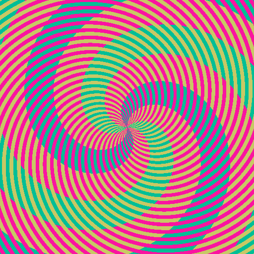
Download the image below. Use the basic image processing tools we learned in class to replace the beige and magenta colors with white and save the resulting image. Display the original image and the altered image side by side. (This problem was inspired by Dan White.)
