Setting up a Python environment for scientific computing
This tutorial was generated from an IPython notebook. You can download the notebook here.
In this tutorial, we will set up a Python computing environment for scientific computing. There are two main ways people do this.
- By downloading and installing package by package with tools like
apt-get,pip, etc. - By downloading and installing a Python distribution that contains binaries of many of the scientific packages needed. The major distributions of these are Python(x,y), Anaconda, and Enthought Canopy. All contain IDEs.
In this class, we will use Enthought Canopy. I have found it very useful for instructional use, though I have also used Anaconda in my research.
Python 2 vs 3
Importantly, Canopy is a distribution that uses Python 2.7 (Anaconda has Python 3 available, but not with optimized performance). Python is currently in version 3.4. Why use 2.7? The answer is that Python 3.x is not backwards compatible with Python 2.x. Boatloads of code are written in Python 2, and the scientific community is notoriously slow in switching to Python 3. I suspect Enthought is keeping Canopy running 2.7 mainly for this reason: there is lots of optimized Python 2.7 code that works very well. I suspect that next year I will teach this course using Python 3, but for now, we will use Python 2.7, and it will work just fine.
You might want to read this nice discussion by Jake Vanderplas, whose blog we will visit from time to time during the course.
Downloading and installing Enthought Canopy
You should install Canopy with Enthought’s Academic License. This will give you access to all modules they have available for free. Prior to getting the license, you will need to set up an account with Enthought using your Caltech email address (you need the .edu to get the Academic license). You can get Canopy for academic use here. You should download the full version of Canopy, not Canopy Express.
Upon downloading a version of Canopy appropriate for your operating system, use Canopy’s installer to install it by following the on-screen instructions. This should involve just a few clicks.
Launching Canopy and using the Package Manager
Upon installation, you can simply launch Canopy by double-clicking the Canopy icon. Upon launch, Canopy will ask you some customization questions. You should select the defaults unless you have a very good reason not to.
After launching, Canopy’s welcome screen will appear. It looks like this:
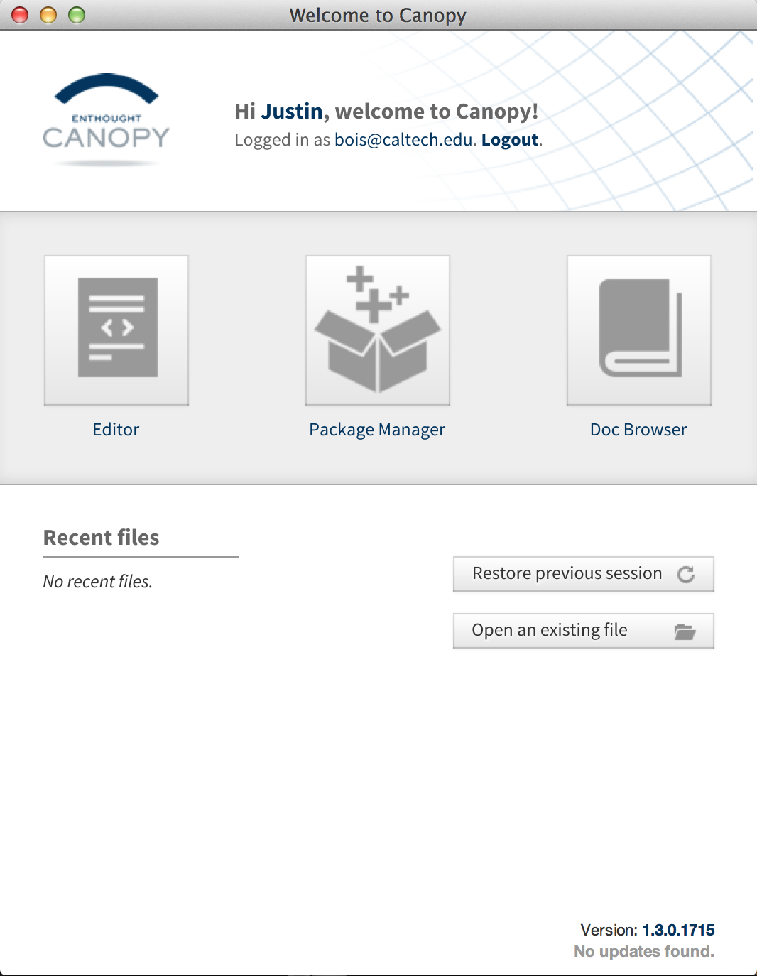
(This image is a bit old; my current version is 1.4.1.1975.)
In the lower right, you can see if there are any Canopy updates available. These are not package updates, but updates for Canopy itself. You can choose to look at documentation with the Doc Browser (which essentially just takes you to documentation websites), manage the packages you have installed and want to install with the Package Manager, or open the Editor, which is where you will compose and execute your Python code.
You should start by clicking on the Package Manager. Then, click “Updates” and “Install all Updates.” This will make all of Canopy’s default packages updated to the current versions.
If you click on “Available Packages,” you can see all the packages that are available for installation. Most of what you need for BE/Bi 103 is already included in the default full Canopy distribution.
Using the Canpoy editor and checking your installation
We will now open Canopy's Editor and use it to test our installation.
From Canopy’s Welcome Screen, click on “Editor.” A default Editor window will open. It looks like this:
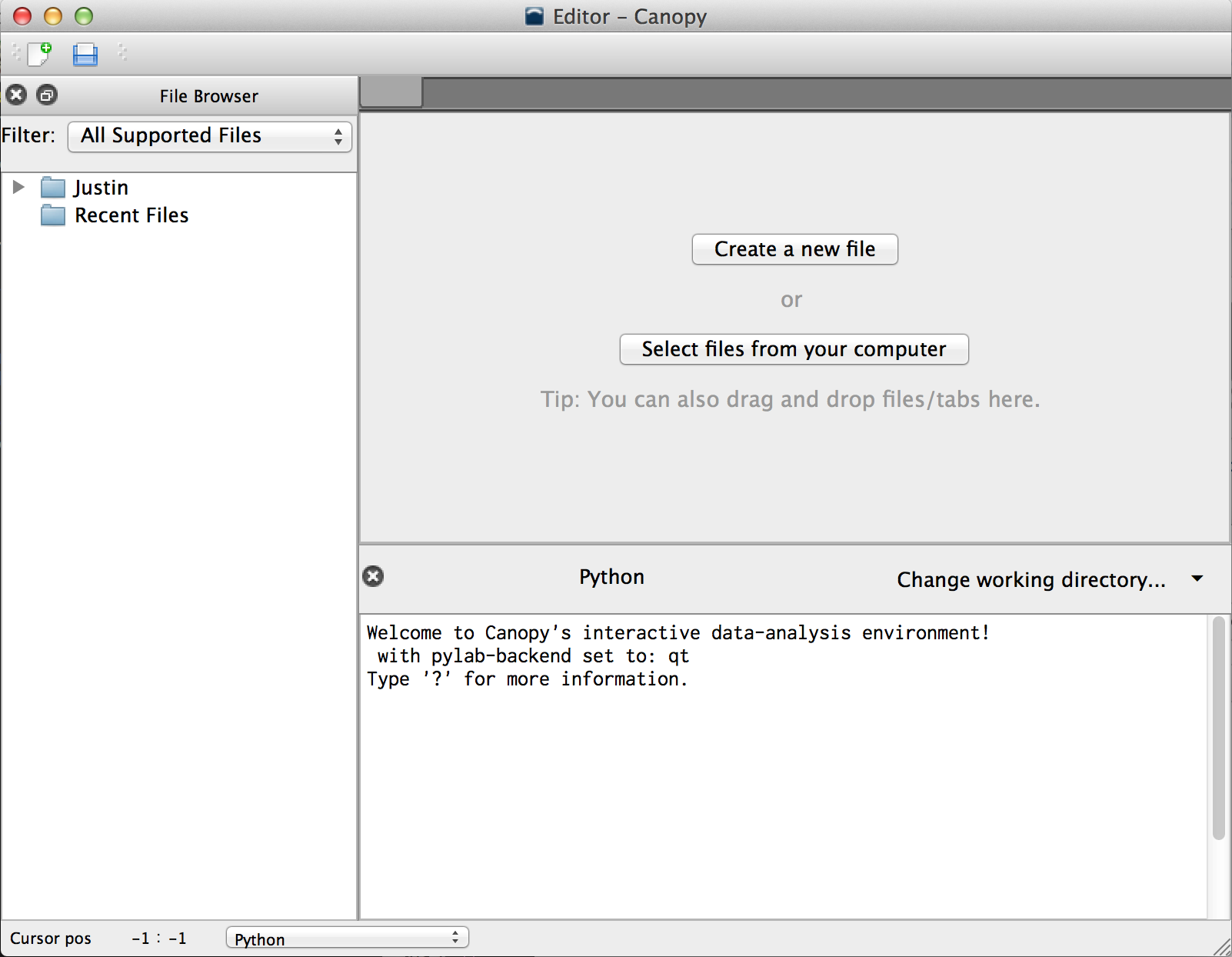
This is where you do most of your work. You can close the File Browser pane if you wish to give yourself more room. You can also resize the respective panes to whatever is comfortable for you.
The Python pane in the Canopy Editor is running IPython. This is an interactive Python shell that is very convenient to use. For example, you can press the up arrow to recall previous commands, and tab completion also works.
Now, we're ready to test if our installation worked. We will generate a plot of the Gamma distribution
\begin{align} f(x~|~a,\lambda) = \frac{(\lambda x)^a\,\mathrm{e}^{-\lambda x}}{x\Gamma(a)} \end{align}
on the domain $0 \le x \le 10$ with $a = 2$ and $\lambda = 1$. So, we're plotting $f(x~|~2,1) = x \mathrm{e}^{-x}$.
In the Python pane, we will execute the following commands at the prompt (skipping the Matplotlib inline command, which is used to generate this document). We will discuss what these commands mean in our first lab session; for now, just enter them (without the comments of course) and see if everything works.
# Do not do this
%matplotlib inline

# Do everything following
import numpy as np
import matplotlib.pyplot as plt

# Generate x values
x = np.linspace(0.0, 10.0, 100)
y = x * np.exp(-x)

# Generate the plot
plt.plot(x, y, 'k-')
plt.margins(0.02, 0.02)
plt.xlabel(r'$x$')
plt.ylabel(r'$y$')

plt.draw()
plt.show()
You should have a window pop up that shows the plot above. If you do, excellent! You now have a functioning Python environment for scientific computing! See you in class!