Tutorial 8a: Particle tracking
This tutorial was generated from an IPython notebook. You can download the notebook here.
In this tutorial, we will track a particle in an XYT stack over time. Our purpose is to calibrate an optical trap, but particle tracking is common in a wide variety of applications. The techniques we cover here have widespread use.
Before we begin, we import our favorite modules, as always.
# As usual, import modules
from __future__ import division, absolute_import, \
                                    print_function, unicode_literals

import os

import numpy as np
import pandas as pd
import scipy.constants
import scipy.optimize
import scipy.signal
import matplotlib.pyplot as plt
from matplotlib import cm

# A whole bunch of skimage stuff
import skimage.feature
import skimage.filter
import skimage.io
import skimage.morphology

# Utilities from JB
import jb_utils as jb

# Necessary to display plots in this IPython notebook
%matplotlib inline
The data set
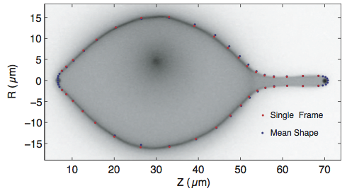
The data were used to calibrate the optical trap used in Lee, et al., Membrane shape as a reporter for applied forces, PNAS, 105, 19253–19257, 2008. The objective in that paper was to determine the externally applied forces, as well as the pressure, tension, and spontaneous curvature of membranes comprising vesciles using shape alone. For example, in the figure below, the authors used two beads in optical traps to stretch a vesicle. They then measured the shape of the vesicle over time and were able to compute the externally applied force from the optical traps. To check their model, they needed to know what the applied force by the optical traps was.
The optical trap is modeled as a "spring", meaning that the force exerted on the bead varies linearly with its displacement from the center of the trap. I.e., if $x = 0$ is the center of the trap, then the force exerted by the trap on the bead is $F = -k x$, where $k$ is the spring constant, called the trap stiffness. This model is value for small displacements from the center of the trap. Our goal is to measure the trap stiffness so we can then use it to compute forces exerted on vesicles.
Other pertinent information about this data set:
- The data were acquired at room temperature, $T = 22\,^\circ$C.
- The time between frames was 60 ms.
- The interpixel distance was 0.28 µm.
- The bead diameter is 1 µm.
Given these values, it is useful to store them for future use. The temperature does not come directly into any calculations, except through the thermal energy, $kT$. We will work in units where force is in units of pN, lengths are in units of µm, and time in units of seconds.
# Thermal energy, kT, in units of pN-µm
kT = scipy.constants.k * (273.15 + 22.0) * 1e18

# Bead radius in units of µm
a = 0.5

# Interpixel distance in units of microns
physical_size = 0.28

# Time between frames in units of seconds
dt = 0.06
Trap calibration using the equipartition theorem
Perhaps the simplest way to calibrate the optical trap is to use a classic result from statistical mechanics, the equipartition theorem. The theorem states that for every degree of freedom $x$ that enters into the Hamiltonian of a system as a quadratic potential, $H_x = \frac{1}{2}kx^2$, $\langle H_x\rangle = \frac{1}{2}k_\mathrm{B}T$. This is easier understood by deriving it. The energy of the bead in the trap as a function of position is Boltzmann distributed, so the average energy is
\begin{align} \left<H_x\right> = \frac{1}{Z}\int_{-\infty}^\infty \mathrm{d}x\,H_x\mathrm{e}^{-\beta H_x}, \end{align}
where $\beta = 1/k_\mathrm{B}T$, and $Z$ is the partition function, given by
\begin{align} Z = \int_{-\infty}^\infty \mathrm{d}x\,\mathrm{e}^{-\beta H_x}. \end{align}
We can compute the partition function and $\langle H_x \rangle$ using Gaussian integrals.
\begin{align} \left<H_x\right> &= \frac{1}{Z}\frac{k}{2}\int_{-\infty}^\infty \mathrm{d}x\,x^2\mathrm{e}^{-\beta k x^2/2} = \frac{k}{2Z}\sqrt{\frac{2\pi}{(\beta k)^3}} \\[1mm] Z &= \int_{-\infty}^\infty \mathrm{d}x\,\mathrm{e}^{-\beta k x^2/2} = \sqrt{\frac{2\pi}{\beta k}}. \end{align}
Putting these together gives
\begin{align} \langle H_x\rangle = \frac{k}{2} \langle x^2 \rangle = \frac{1}{2}k_\mathrm{B}T. \end{align}
We will use this last equality to compute the trap stiffness, $k$.
\begin{align} k = \frac{k_\mathrm{B}T}{\langle x^2 \rangle}. \end{align}
In other words, we will compute the mean square displacement of the bead from the center of the trap to compute $k$.
Loading in the trapped images
We'll start by loading in the freely diffusing particle.
# Load in stack (don't need to conserve memory)
trap_xyt = jb.XYTStack(directory='../data/lee_et_al/trapped/',
                       conserve_memory=False, dt=dt,
                       physical_size_x=physical_size,
                       physical_size_y=physical_size)
There is a new function in jb_utils to view movies stored in an XYTStack object. It will not work here in an IPython notebook without some extra work, so I will not do it here. But to view a movie of the bead in the trap, do the following.
# To view movie, uncomment below
# trap_xyt.show_movie()
Finding the center of the bead to pixel accuracy
Let's look at a single image of a particle in the trap.
# Display image of bead in trap
plt.imshow(trap_xyt.im(0), cmap=cm.gray)
We can easily find the center of the particle by finding the pixel in this image with the highest intensity.
# np.argmax gives index of maximum in flattened array
peak_flat_ind = np.argmax(trap_xyt.im(0))

# Convert flattened array value to i, j
peak_j = peak_flat_ind % trap_xyt.size_x
peak_i = (peak_flat_ind - peak_j) / trap_xyt.size_x

# Highlight this pixel in the image
plt.imshow(trap_xyt.im(0), cmap=cm.gray)
plt.plot(peak_j, peak_i, 'r.')
plt.xlim((0, trap_xyt.size_x))
plt.ylim((0, trap_xyt.size_y));
This technique is useful for these images with a single bead, but if we want to find more particles to track in other applications, this will not work. For an application like that, we can use skimage.feature.peak_local_max. When doing this, it is often better to perform a light Gaussian blur first.
# Get particle size in pixels
particle_size_pix = 2 * a / trap_xyt.physical_size_x

# Perform Gaussian blur
im_blur = skimage.filter.gaussian_filter(trap_xyt.im(0), 2.0)

# Threshold value the pixel value must exceed to be peak
thresh = im_blur.mean() + 2.0 * im_blur.std()

# Find peaks using peak finder
peaks = skimage.feature.peak_local_max(
    im_blur, min_distance=particle_size_pix, threshold_abs=thresh)

# Show result
plt.imshow(im_blur, cmap=cm.gray)
plt.plot(peaks[:,1], peaks[:,0], 'r.')
plt.xlim((0, trap_xyt.size_x))
plt.ylim((0, trap_xyt.size_y));
Finding the bead center with subpixel accuracy
As can be seen from the movie, the bead does not move much in the trap. So, we need to find its position to subpixel accuracy. To do this, we will employ a nine-point estimate in which we take the nine-point neighborhood around the pixel with highest intensity and fit the pixel intensities to a symmetric 2D Gaussian. The best way to do this is still an area of active research. For large data sets, speed can be very important. We will take the computationally expensive but simple approach of directly fitting the 2D Gaussian. The local image is described by
\begin{align} I(x,y) = a \, \exp\left\{-\frac{(x-x_0)^2 + (y-y_0)^2}{2\sigma^2}\right\}. \end{align}
The center of the bead is given by $(x_0, y_0)$.
In the code that follows, I actually allow for any structuring element to be used in the fitting, but in practice, most people use the nine-point estimate.
We start by writing a function to fit a symmetric Gaussian to a neighborhood of pixel values.
# Fit symmetric Gaussian to x, y, z data
def fit_gaussian(x, y, z):
    """
    Fits symmetric Gaussian to x, y, z.

    Fit func: z = a * exp(-((x - x_0)**2 + (y - y_0)**2) / (2 * sigma**2))

    Returns: p = [a, x_0, y_0, sigma]
    """

    def sym_gaussian(p):
        """
        Returns a Gaussian function:
        a**2 * exp(-((x - x_0)**2 + (y - y_0)**2) / (2 * sigma**2))
        p = [a, x_0, y_0, sigma]
        """
        a, x_0, y_0, sigma = p
        return a**2 \
                * np.exp(-((x - x_0)**2 + (y - y_0)**2) / (2.0 * sigma**2))

    def sym_gaussian_resids(p):
        """Residuals to be sent into leastsq"""
        return z - sym_gaussian(p)

    def guess_fit_gaussian():
        """
        return a, x_0, y_0, and sigma based on computing moments of data
        """
        a = z.max()

        # Compute moments
        total = z.sum()
        x_0 = np.dot(x, z) / total
        y_0 = np.dot(y, z) / total

        # Approximate sigmas
        sigma_x = np.dot(x**2, z) / total
        sigma_y = np.dot(y**2, z) / total
        sigma = np.sqrt(sigma_x * sigma_y)

        # Return guess
        return (a, x_0, y_0, sigma)

    # Get guess
    p0 = guess_fit_gaussian()

    # Perform optimization using nonlinear least squares
    popt, junk_output, info_dict, mesg, ier = \
            scipy.optimize.leastsq(sym_gaussian_resids, p0, full_output=True)

    # Check to make sure leastsq was successful.  If not, return centroid
    # estimate.
    if ier in (1, 2, 3, 4):
        return (popt[0]**2, popt[1], popt[2], popt[3])
    else:
        return p0
With our Gaussian fitting function in hand, we can write another function to get the position of the bead (in units of pixels).
def bead_position_pix(im, selem):
    """
    Determines the position of bead in image in units of pixels with
    subpixel accuracy.
    """
    # The x, y coordinates of pixels are nonzero values in selem
    y, x = np.nonzero(selem)
    x = x - selem.shape[1] // 2
    y = y - selem.shape[0] // 2

    # Find the center of the bead to pixel accuracy
    peak_flat_ind = np.argmax(im)
    peak_j = peak_flat_ind % im.shape[0]
    peak_i = (peak_flat_ind - peak_j) // im.shape[1]

    # Define local neighborhood
    irange = (peak_i - selem.shape[0] // 2, peak_i + selem.shape[0] // 2 + 1)
    jrange = (peak_j - selem.shape[1] // 2, peak_j + selem.shape[1] // 2 + 1)

    # Get values of the image in local neighborhood
    z = im[irange[0]:irange[1], jrange[0]:jrange[1]][selem.astype(np.bool)]

    # Fit Gaussian
    a, j_subpix, i_subpix, sigma = fit_gaussian(x, y, z)

    # Return x-y position
    return np.array([peak_i + i_subpix, peak_j + j_subpix])
We now have the machinery in place to get the position of the bead to subpixel accuracy.
# We will use the nine-point estimate (as is typically done)
selem = skimage.morphology.square(3)

# Loop through and find centers
centers = []
for i in range(trap_xyt.size_t):
    centers.append(bead_position_pix(trap_xyt.im(i), selem))

# Store as NumPy array
centers = np.array(centers)
Now that we have the centers of the bead for each frame, we just need to compute the displacements in $x$ and $y$.
# Get displacements
x = centers[:,1] - centers[:,1].mean()
y = centers[:,0] - centers[:,0].mean()

# Plot displacement
plt.plot(trap_xyt.t, x, lw=1, zorder=1, label=r'$x$')
plt.plot(trap_xyt.t, y, lw=0.5, zorder=0, label=r'$y$')
plt.xlabel('time (s)')
plt.ylabel('$x$, $y$ (pixels)')
plt.legend(loc='lower left')
Notice that the bead only moves in subpixel amounts, so the subpixel accuracy of our positional determination was crucial. We also see that the trap is stiffer in the $x$-direction than in $y$. We can use equipartition to compute the trap stiffness in $x$ and $y$.
# Get x and y in real units
x_micron = x * trap_xyt.physical_size_x
y_micron = y * trap_xyt.physical_size_y

# Get k's from equipartition
k_x = kT / (x_micron**2).mean()
k_y = kT / (y_micron**2).mean()

# Print result
print('k_x = %.2f pN/µm' % k_x)
print('k_y = %.2f pN/µm' % k_y)
We will talk about how to get error bars on $k_x$ and $k_y$ in the next lecture. For now, we have values of the trap stiffness.
Trap stiffness from power spectral density
Another common method for computing the trap stiffness it to use the power spectral density of the displacement. The power spectral density, $S_{xx}$ is related to the Fourier transform of the displacements over time. Specifically,
\begin{align} S_{xx}(f) = \left|\hat{x}(f)\right|^2, \end{align}
where $f$ is the frequency and $\hat{x}$ is the Fourier transform of the displacements. Computing the power spectral density for real data is challenging. In particular, we have to pick values of $f$ for which to sample the $S_{xx}$. A convenient method for this is Welch's method. We will not go into the details here, and will use its implementation in scipy.signal.welch.
As worked out long ago by Uhlenbeck, for a particle undergoing thermal motion in a harmonic potential (like out optical trap), the power spectral density has a Lorentzian form.
\begin{align} S_{xx}(f) = \frac{k_\mathrm{B}T}{\pi^2\beta\left(f_0^2 + f^2\right)}, \end{align}
where $\beta$ is the hydrodynamic drag coefficient. (I know this is confusing with $\beta$ also being defined a $1/k_\mathrm{B}T$, but I want to stay consistent with the literature.) The value of the rolloff frequency, $f_0$ is $f_0 = k/2\pi\beta$. So, if we know $\beta$ and can perform a regression to get $f_0$, we can compute $k$.
Computation of hydrodynamic drag
To compute the hydrodynamic drag, we can do an experiment where the trap is shut off and we track the bead. We can then use the fluctuation-dissipation theorem, another beautiful result from statistical mechanics (derived by no less than Albert Einstein) that
\begin{align} D = \frac{k_\mathrm{B}T}{\beta}, \end{align}
where $D$ is the diffusion coefficient for the bead. This can be calculated from the mean square displacement of the particle,
\begin{align} \mathrm{MSD}(\tau) \equiv \langle \left(\mathbf{r}(\tau)\right)^2 \rangle = 2 d D \tau, \end{align}
where $\tau$ is the length of the time interval over which the MSD is computed, and $d$ is the dimensionality of the motion. In our case, we will look at 2D images, so $d = 2$.
So, our strategy is to track a freely diffusing bead over time, compute its MSD over time, perform a regression to get the diffusion coefficient $D$, and then use the fluctuation dissipation theorem to get $\beta$.
We'll start by loading in the images and computing the position of the bead.
# Load in stack (don't need to conserve memory)
diff_xyt = jb.XYTStack(directory='../data/lee_et_al/free_diffusion/',
                       conserve_memory=False, dt=dt,
                       physical_size_x=physical_size,
                       physical_size_y=physical_size)

# Compute bead center as before
selem = skimage.morphology.square(3)

# Loop through and find centers
centers = []
for i in range(diff_xyt.size_t):
    centers.append(bead_position_pix(diff_xyt.im(i), selem))

# Store as NumPy array
centers = np.array(centers)
Now that we have the bead centers, we need to compute the MSD as a function of time windows, $\tau$. Diffusion is a memoryless process, so it does not matter where in the trace we start the time window. Therefore, for a trace with 500 time points, we have 50 independent time intervals containing 10 frames. We could consider overlapping time intervals, but there are some fancy statistics that we would need to do to correct for breaking statistical independence. Instead, we will do what is usually done and only consider independent windows. We will write a function to do this calculation.
# Compute MSD as a function of time interval tau (in units of frames)
def msd_from_trace(x, y=None):
    """
    Assumes constant time interval between frames.

    Definitely not the fastest way to compute MSDs.
    """
    # Number of data points
    n = len(x)

    # Set up time windows and number of intervals averaged in each
    ind_diff = np.arange(4, n // 8)
    n_windows = len(ind_diff)
    n_points_averaged = n // ind_diff - 1

    # Set up array of MSDs and errors
    msd = np.empty(n_windows)
    msd_err = np.empty(n_windows)

    # Loop over interval lengths
    for i in range(n_windows):
        t = ind_diff[i]
        msds = np.empty(n_points_averaged[i])

        # Loop over all nonoverlapping windows with interval length
        for j in range(0, n_points_averaged[i]):
            k = j * t
            msds[j] = (x[k + t] - x[k])**2
            if y is not None:
                msds[j] += (y[k + t] - y[k])**2

        # Compute mean and s.e.m. for interval length
        msd[i] = msds.mean()
        msd_err[i] = msds.std() / np.sqrt(n_points_averaged[i])

    return ind_diff, msd, msd_err
With this in hand, we can compute the MSDs. We'll convert from units of pixels to real lengths.
# Convert positions from pixels to real length
x = centers[:,1] * diff_xyt.physical_size_x
y = centers[:,0] * diff_xyt.physical_size_y

# Compute MSDs from trace of bead position
tau_ind, msd, msd_err = msd_from_trace(x, y)

# Convert intervals to real time
tau = tau_ind * diff_xyt.dt
We can now plot our MSD vs. $\tau$.
# Plot results
plt.errorbar(tau, msd, yerr=msd_err, ls='none', color='k', elinewidth=1)
plt.xlabel(r'$\tau$ (s)')
plt.ylabel(r'$\langle \mathbf{r}^2 \rangle$ (µm$^2$)');
We now just have to fit this with a linear function,
\begin{align} \mathrm{MSD}(\tau) = 4D\tau. \end{align}
This is now old hat for us! Since we are going to be flippant with error bars, we will just assume a uniform prior.
# Define our function to pass to scipy.optimize.curve_fit
def linear(tau, diff_coeff):
    return 4.0 * diff_coeff * tau

# Define log of posterior
def log_posterior(diff_coeff, tau, msd, msd_err):
    return -((msd - linear(tau, diff_coeff[0]))**2 / msd_err**2).sum()

# Generate an initial guess to put into the solver
p0 = np.array([10.0])

# Fit fixed width bins
p_opt, junk_output = scipy.optimize.curve_fit(linear, tau, msd, p0,
                                              sigma=msd_err)

# Compute error bar
var = -1.0 / jb.hess_nd(log_posterior, p_opt, (tau, msd, msd_err))[0,0]

# Extract results
diff_coeff = p_opt[0]
diff_coeff_err = np.sqrt(var)

# Print results
print('D = %.2f +- %.2f µm^2/s' % (diff_coeff, diff_coeff_err))

# Plot results
tau_smooth = np.array([0.0, 4.0])
msd_smooth = linear(tau_smooth, diff_coeff)
plt.errorbar(tau, msd, yerr=msd_err, ls='none', color='k', elinewidth=1)
plt.plot(tau_smooth, msd_smooth, 'r-')
plt.xlabel(r'$\tau$ (s)')
plt.ylabel(r'$\langle \mathbf{r}^2 \rangle$ (µm$^2$)')
Using the fluctuation dissipation theorem, we can now compute $\beta$.
# Compute beta
beta = kT / diff_coeff

# Print result
print('beta = %.4f pN-s/µm' % beta)
As a check, we can compare this result to what we would expect from Stokes law, which gives
\begin{align} \beta = 6\pi\eta a, \end{align}
where $\eta \approx 0.89$ cP $= 0.00089$ pN-s/µm$^2$.
# Compute eta from beta
eta = beta / 6.0 / np.pi / a

# Print result
print('eta = %.3f cP' % (eta * 1000))
Fitting the power spectral density
With $\beta$ in hand, we can fit the power spectral density. In order to measure the power spectral density, we need very high frame rate measurements of the bead position. This is achieved by using a position sensitive device that is attached to the optics of the system (and confusingly also has the initials PSD). The PSD measures voltage on a detector for high light intensity, which enables measurement of position. The voltage in the $x$-channel is proportional to the $x$-position and similarly for $y$. For the measurements in this data set, the sampling rate was $10^4$ Hz.
The trace is split into several files with 3000 samples each. If I recall correctly from my conversations with Heun Jin Lee, who acquired these data, this was to enable high-speed saving of the data. We will piece these files together into a single signal.
# Get a list of the CSV files
psd_prefix = '../data/lee_et_al/psd_data'
csv_files = os.listdir(psd_prefix)

# Make empty lists for x and y voltage
x = []
y = []

# Load each CSV file and append
for fname in csv_files:
    full_fname = os.path.join(psd_prefix, fname)
    psd_data = pd.read_csv(full_fname)
    x.append(psd_data.x.values)
    y.append(psd_data.y.values)

# Make single NumPy arrays for results
x = np.concatenate(x)
y = np.concatenate(y)

# Subtract the mean to get displacement
x = x - x.mean()
y = y - y.mean()

# Plot the results (only every 1000ths point)
t = np.arange(len(x)) / 10000.0
plt.plot(t[::1000], y[::1000], 'g-', lw=0.25, zorder=0)
plt.plot(t[::1000], x[::1000], 'b-', lw=0.5, zorder=1)
plt.xlim((t.min(), t.max()));
We have an expression for $S_{xx}$, but we can only compute $S_{vv}$, the voltage power spectrum, from the data. However, because they are proportional, we can write
\begin{align} S_{vv} = \frac{c}{f_0^2 + f^2}, \end{align}
where $c$ is some constant. So, we go ahead and use Welch's method to compute the power spectral density $S_{vv}$.
# Compute PSD
f_x, psd_x = scipy.signal.welch(x, 10000.0)
f_y, psd_y = scipy.signal.welch(y, 10000.0)

# High f scaling
f_high = np.array([1e2, 1e4])
p_scaling = 1e-2/ f_high**2

# Plot result
plt.loglog(f_x, psd_x, 'k.', label='$x$')
plt.loglog(f_y, psd_y, 'r.', label='$y$')
plt.loglog(f_high, p_scaling, 'k--')
plt.ylabel(r'S_{vv} (V$^2\cdot$s$\cdot$µm$^{-2}$)')
plt.xlabel('f (Hz)')
plt.ylim((1e-9, 1e-6))
plt.grid(True)
plt.legend(loc='lower left', numpoints=1);
We already see some problems. First, the curves to not quite reach the expected high frequency scaling of $f^{-2}$ (represented by dashed line) that we expect. We therefore already see a violation of Lorentzian-ness. Second, we barely capture the rolloff frequency in the $y$ channel. We also see that the curve loses its log-linear scaling at hight frequencies. This could be due to bandwidth limitations of the detector; such limitations are documented in the literature. This is a case where we have good reason to believe there is something wrong with the experiment/detector in the high frequency regime, and we may neglect those data. We will therefore only consider frequencies up to 2000 Hz.
It is the log of the power spectrum that is relevant, so we will fit
\begin{align} \ln S_{vv}(f) = \ln c - \ln\left(f_0^2 + f^2\right). \end{align}
We have not properly computed the error bar in $\beta$, so we will not bother with computing an error bar on our rolloff frequency $f_0$ or the trap stiffness $k$.
# Define our function to pass to scipy.optimize.curve_fit
def log_lorentzian(f, f_0, c):
    return c - np.log(f_0**2 + f**2)

# Generate an initial guess to put into the solver
p0 = np.array([300.0, -3.0])

# Only consider frequencies less than 2000 Hz
inds_x = f_x < 2000
inds_y = f_y < 2000

# Fit fixed width bins
p_opt_x, junk_output = scipy.optimize.curve_fit(log_lorentzian, f_x[inds_x],
                                                np.log(psd_x[inds_x]), p0)
p_opt_y, junk_output = scipy.optimize.curve_fit(log_lorentzian, f_y[inds_y],
                                                np.log(psd_y[inds_y]), p0)

# Extract results
f_0_x = p_opt_x[0]
c_x = p_opt_x[1]
f_0_y = p_opt_y[0]
c_y = p_opt_y[1]

# Plot results
f_smooth = np.logspace(1, 4, 100)
psd_x_smooth = np.exp(log_lorentzian(f_smooth, *(p_opt_x)))
psd_y_smooth = np.exp(log_lorentzian(f_smooth, *p_opt_y))

plt.loglog(f_high, p_scaling, 'k--')
plt.loglog(f_x, psd_x, 'k.', label='$x$')
plt.loglog(f_smooth, psd_x_smooth, 'k-')
plt.loglog(f_y, psd_y, 'r.', label='$y$')
plt.loglog(f_smooth, psd_y_smooth, 'r-')
plt.ylabel(r'PSD (V$^2\cdot$s$\cdot$µm$^{-2}$)')
plt.xlabel('f (Hz)')
plt.ylim((1e-9, 1e-6))
plt.grid(True)
plt.legend(loc='lower left', numpoints=1);
From the regression, we can use $k = 2\pi \beta f_0$ to compute the trap stiffness.
# Compute trap stiffness
k_x = 2.0 * np.pi * beta * f_0_x
k_y = 2.0 * np.pi * beta * f_0_y

# Print results
print("""
k_x = {0:.2f} pN/µm
k_y = {1:.2f} pN/µm
""".format(k_x, k_y))
These regressions do not pass the eye test; the spectra do not appear to be Lorentzian. Nonetheless, they give roughly the same order of magnitude as using the equipartition theorem. Of course, order of magnitude for the trap stiffness is not enough for precise force measurements!