BE/Bi 103, Fall 2016: Homework 4

Due 1pm, Sunday, October 23

(c) 2016 Justin Bois. This work is licensed under a Creative Commons Attribution License CC-BY 4.0. All code contained therein is licensed under an MIT license.

This homework was generated from an Jupyter notebook. You can download the notebook here.

import numpy as np
import numba

Problem 4.1: Writing your own MCMC sampler (60 pts + 40 pts extra credit)

a) Write your own MCMC sampler that employs a Metropolis-Hastings algorithm that uses a Gaussian proposal distribution. Since you are sampling multiple parameters, your proposal distribution will be multi-dimensional. You can use a Gaussian proposal distribution with a diagonal covariance. In other words, you generate a proposal for each variable in the posterior independently.

You can organize your code how you like, but here is a suggestion.

• Write a function that takes (or rejects) a Metropolis-Hastings step. It should look something like the below (obviously where it does something instead of passing).

def mh_step(x, log_post, logpost_current, sigma, args=()):
    """
    Parameters
    ----------
    x : ndarray, shape (n_variables,)
        The present location of the walker in parameter space.
    log_post : function
        The function to compute the log posterior. It has call
        signature `log_post(x, *args)`.
    log_post_current : float
        The current value of the log posterior.
    sigma : ndarray, shape (n_variables, )
        The standard deviations for the proposal distribution.
    args : tuple
        Additional arguments passed to `log_post()` function.

    Returns
    -------
    x_out : ndarray, shape (n_variables,)
        The position of the walker after the Metropolis-Hastings
        step. If no step is taken, returns the inputted `x`.
    log_post_updated : float
        The log posterior after the step.
    accepted : bool
        True is the proposal step was taken, False otherwise.
    """
    
    pass

• Write another function that calls that function over and over again to do the sampling. It should look something like this:

def mh_sample(log_post, x0, sigma, args=(), n_burn=1000, n_steps=1000,
              variable_names=None):
    """
    Parameters
    ----------
    log_post : function
        The function to compute the log posterior. It has call
        signature `log_post(x, *args)`.
    x0 : ndarray, shape (n_variables,)
        The starting location of a walker in parameter space.
    sigma : ndarray, shape (n_variables, )
        The standard deviations for the proposal distribution.
    args : tuple
        Additional arguments passed to `log_post()` function.
    n_burn : int, default 1000
        Number of burn-in steps.
    n_steps : int, default 1000
        Number of steps to take after burn-in.
    variable_names : list, length n_variables
        List of names of variables. If None, then variable names
        are sequential integers.
    
    Returns
    -------
    output : DataFrame
        The first `n_variables` columns contain the samples.
        Additionally, column 'lnprob' has the log posterior value
        at each sample.
    """
    
    pass

b) To test your code, we will get samples out of a known distribution. We will use a bivariate Gaussian with a mean of $\boldsymbol{\mu} = (10, 20)$ and covariance matrix of

\begin{align} \boldsymbol{\sigma} = \begin{pmatrix} 4 & -2 \\ -2 & 6 \end{pmatrix} \end{align}

I have written the function to be unnormalized and JITted with numba for optimal speed.

Do not be confused: In this test function we are sampling $\mathbf{x}$ out of $P(\mathbf{x}\mid \boldsymbol{\mu},\boldsymbol{\sigma})$. This is not sampling a posterior; it's just a test for your code. You will pass log_test_distribution as the log_post argument in the above functions.

mu = np.array([10.0, 20])
cov = np.array([[4, -2],[-2, 6]])
inv_cov = np.linalg.inv(cov)

@numba.jit(nopython=True)
def log_test_distribution(x, mu, inv_cov):
    """
    Unnormalized log posterior of a multivariate Gaussian.
    """
    return -np.dot((x-mu), np.dot(inv_cov, (x-mu))) / 2

If you compute the means and covariance (using np.cov()) of your samples, you should come close to the inputed means and covariance. You might also want to plot your samples using corner.corner() to make sure everything makes sense.

c) (20 pts extra credit) Add in some logic to your Metropolis-Hastings sampler to enable tuning. This is the process of automatically adjusting the $\sigma$ in the proposal distribution such that the acceptance rate is desirable. The target acceptance rate is about 0.4. The developers of PyMC3 use the scheme below, which is reasonable.

Acceptance rate	Standard deviation adaptation
< 0.001	$\times$ 0.1
< 0.05	$\times$ 0.5
< 0.2	$\times$ 0.9
> 0.5	$\times$ 1.1
> 0.75	$\times$ 2
> 0.95	$\times$ 10

Be sure to test your code to demonstrate that it works.

d) (20 pts extra credit) Either adapt the functions you already wrote or write new ones to enable sampling of discrete variables. Again, be sure to test your code.

Problem 4.2: MCMC with Boolean data (40 pts)

In this problem, we will work with data of the True/False type. Lots of data sets in the biological sciences are like this. For example, we might look at a certain mutation in Drosophila that affects development and we might check whether or not eggs hatch.

The data we will use comes from an experiment we did the last couple years in Bi 1x here at Caltech. The experiment was developed by Meaghan Sullivan. We studies a neural circuit in C. elegans using optogenetics.

A neural circuit is a series of interconnected neurons that create a pathway to transmit a signal from where it is received, to where it causes a behavioral response in an animal. An example is the neural circuit involved in reversals in C. elegans. This circuit consists of three types of neurons: sensory neurons receive stimuli from the environment, command interneurons integrate information from many sensory neurons and pass a signal to the motor neurons, and motor neurons control worm behavior, such as reversals.

There are six neurons acting in a circuit that responds to environmental cues and triggers a reversal, a shown in the figure below (based on Schultheis et. al. 2011). These include four sensory neurons (ALM, AVM, ASH, and PLM). Each sensory neuron is sensitive to a different type of stimulus. For example, the sensory neuron we are studying (ASH) is sensitive to chemosensory stimuli such as toxins, while another neuron (PLM) is sensitive to mechanical stimuli (touch) in the posterior part of the worm's body. The sensory neurons send signals that are integrated by two command interneurons (AVA and AVD). Each sensory neuron can provide an impulse to the command interneurons at any time. In order for the command interneuron to fire and activate motor neurons, the sum of the stimuli at any point in time must exceed a certain threshold. Once the stimuli from one or more sensory neurons has induced an action potential in a command interneuron, that signal is passed to motor neurons which will modulate worm behavior.

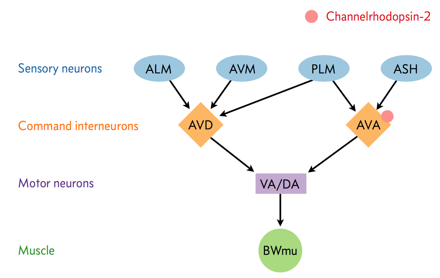
In the experiment, we used optogenetics to dissect the function of individual neurons in this circuit. We worked with two optogenetic worm strains. The ASH strain has channelrhodopsin (ChR2, represented by a red barrel in the figure above) expressed only in the ASH sensory neuron. When we shine blue light on this strain, we should activate the ChR2, which will allow sodium and calcium cations to flow into the neuron, simulating an action potential. We want to quantify how robustly this stimulation will cause the worm to exhibit aversion behavior and reverse.

We also studied an AVA strain that has channelrhodopsin expressed only in the AVA command interneuron. Our goal is to quantify the effects of stimulating this neuron in terms of reversals compared to the ASH neuron and to wild type.

The True/False data here are the whether or not the worms undergo a reversal. Here is what the students observed.

Strain	Year	Trials	Reversals
WT	2016	36	6
ASH	2016	35	12
AVA	2016	36	30
WT	2015	35	0
ASH	2015	35	9
AVA	2015	36	33

For the purposes of this problem, assume that we can pool the results from the two years to have 6/71 reversals for wild type, 21/70 reversals for ASH, and 63/72 reversals for AVA.

Our goal is to estimate $p$, the probability of reversal for each strain. That is to say, we want to compute $P(p\mid r, n, I)$, where $r$ is the number of reversals in $n$ trials.

a) Write down an expression for the posterior distribution. That is, write down an expression for the likelihood and prior. You can actually compute the evidence analytically, but that is not necessary for this problem; you can just write down the likelihood and prior.

b) Use your Metropolis-Hastings sampler to sample this posterior for $p$ for each of the three strains. If you were unable to compute problem 3.1, you may use emcee to do the sampling. Plot the results. Do you think there is a difference between the wild type and ASH? How about between ASH and AVA?

c) The posterior plots from part (b) are illuminating, but suppose we want to quantify the difference in reversal probability between the two strains, say strain 1 and strain 2. That is, we want to compute $P(\delta\mid D, I)$, where $\delta \equiv p_2 - p_1$. Use MCMC to compute this, employing your Metropolis-Hastings solver if you can, using emcee otherwise.

After you have done that with MCMC, it is useful to look at what a pain it is to attempt it analytically. I am just showing this as a lesson to you. To compute the distribution $P(\delta\mid D, I)$, we use the fact that we can easily compute the joint probability distribution because the two strains are independent. To ease notation, we will note that the prior $P(p_1, p_2\mid I)$ is only nonzero if $0\le p_1,p_2 \le 1$, instead of writing it explicitly. The posterior is

\begin{align} P(p_1, p_2\mid D, I) &= \frac{(n_1+1)!\,(n_2+1)!}{(n_1-n_{r1})!\,n_{r1}!\,(n_2 - n_{r2})!\,n_{r2}!} \\[0.5em] &\;\;\;\;\;\;\;\;\times\,p_1^{n_{r1}}\,(1-p_1)^{n_1-n_{r1}}\,p_2^{n_{r2}}\,(1-p_2)^{n_2-n_{r2}}. \end{align}

We can define new variables $\delta = p_2 - p_1$ and $\gamma = p_1 + p_2$. Then, we have $p_1 = (\gamma - \delta) / 2$ and $p_2 = (\gamma + \delta) / 2$. Again, to ease notation, we note that $P(\gamma, \delta\mid D, I)$ is nonzero only when $-1 \le \delta \le 1$ and $|\delta| \le \gamma \le 2 - |\delta|$. By the change of variables formula for probability distributions we have

\begin{align} P(\gamma, \delta \mid D, I) = \begin{vmatrix} \mathrm{d}p_1/\mathrm{d}\gamma & \mathrm{d}p_1/\mathrm{d}\delta \\ \mathrm{d}p_2/\mathrm{d}\gamma & \mathrm{d}p_2/\mathrm{d}\delta \end{vmatrix} P(p_1, p_2 \mid n_{r1}, n_{r2}, n_1, n_2, I) = \frac{1}{2}\,P(p_1, p_2 \mid D, I). \end{align}

Thus, we have

\begin{align} P(\gamma, \delta\mid D, I) &= \frac{(n_1+1)!\,(n_2+1)!}{2(n_1-n_{r1})!\,(n_2-n_{r2})!\,n_1!\,n_2!} \\ &\;\;\;\;\times \left(\frac{\gamma-\delta}{2}\right)^{n_{r1}}\,\left(1-\frac{\gamma-\delta}{2}\right)^{n_1-n_{r1}} \left(\frac{\gamma+\delta}{2}\right)^{n_{r2}}\,\left(1-\frac{\gamma+\delta}{2}\right)^{n_2-n_{r2}}. \end{align}

Finally, to find $P(\delta\mid D, I)$, we marginalize by integrating over all possible values of $\gamma$.

\begin{align} P(\delta\mid D, I) = \int_{|\delta|}^{2-|\delta|}\mathrm{d}\gamma\, P(\gamma, \delta\mid D, I) \end{align}

We can expand each of the multiplied terms in the integrand into a polynomial using the binomial theorem, and can then multiply the polynomials together to get a polynomial expression for the integrand. This can then be integrated. There is a technical term describing this process: a big mess. Ouch. This is a major motivation for using MCMC!