BE/Bi 103, Fall 2017: Homework 3
Due 1pm, Sunday, October 15
(c) 2017 Justin Bois. With the exception of the images, this work is licensed under a Creative Commons Attribution License CC-BY 4.0. All code contained therein is licensed under an MIT license.
This homework was generated from an Jupyter notebook. You can download the notebook here.
import pandas as pd
Problem 3.1: Error propagation (10 pts)
Often times, our colleagues do not provide us with full data sets in papers. Say you read two papers, each measuring the same property under putatively the same conditions. One paper reports an estimate of a parameter $\mu$ as $\mu_1 \pm \sigma_1$ and the other reports a value of $\mu_2 \pm \sigma_2$. Based only on this information, what is the most probable value of $\mu$, and what is its error bar?
Problem 3.2: Validating fish activity data (50 pts)
Write some functions to validate the fish activity data set that you can download here. Describe what tests you chose and why you chose them. Run your validation and report on any errors you see.
A bit of background on the data set. These data were acquired by Grigorios Oikonomou in David Prober's lab. The assay is similar to what we saw in Tutorial 2. These fish have mutations in a different gene, the identity of which is not important for this exercise. The data set is unpublished, and at the wishes of the author is password protected.
The file 150717_2A_genotype_3.txt is a genotype file giving the genotypes of the fish in the different locations. Only the fish in instrument 2A, numbered 1 through 96 in the activity data file 150717_2A_2B.csv, were genotyped. The fish in instrument 2B, numbered 97 and above, are not used in the assay.
The instrument give data as MS Excel spread sheets. I have converted the Excel sheet to a CSV file, 150717_2A_2B.csv, but have otherwise not touched it. The columns frect, fredur, midct, middur, burct, and burdur contain information about the fish's activity per minute of observation. The middur columns is what we use for computing activity. For the purposes of this problem, you may ignore the frect, fredur, midct, burct, and burdur columns.
Problem 3.3: Posteriors of True/False data (40 pts)
In this problem, we will work with data of the True/False type. Lots of data sets in the biological sciences are like this. For example, we might look at a certain mutation in Drosophila that affects development and we might check whether or not eggs hatch.
The data we will use comes from an experiment we did the last couple years in Bi 1x here at Caltech. The experiment was developed by Meaghan Sullivan. We studied a neural circuit in C. elegans using optogenetics.
A neural circuit is a series of interconnected neurons that create a pathway to transmit a signal from where it is received, to where it causes a behavioral response in an animal. An example is the neural circuit involved in reversals in C. elegans. This circuit consists of three types of neurons: sensory neurons receive stimuli from the environment, command interneurons integrate information from many sensory neurons and pass a signal to the motor neurons, and motor neurons control worm behavior, such as reversals.
There are six neurons acting in a circuit that responds to environmental cues and triggers a reversal, a shown in the figure below (based on Schultheis et. al. 2011). These include four sensory neurons (ALM, AVM, ASH, and PLM). Each sensory neuron is sensitive to a different type of stimulus. For example, the sensory neuron we are studying (ASH) is sensitive to chemosensory stimuli such as toxins, while another neuron (PLM) is sensitive to mechanical stimuli (touch) in the posterior part of the worm's body. The sensory neurons send signals that are integrated by two command interneurons (AVA and AVD). Each sensory neuron can provide an impulse to the command interneurons at any time. In order for the command interneuron to fire and activate motor neurons, the sum of the stimuli at any point in time must exceed a certain threshold. Once the stimuli from one or more sensory neurons has induced an action potential in a command interneuron, that signal is passed to motor neurons which will modulate worm behavior.
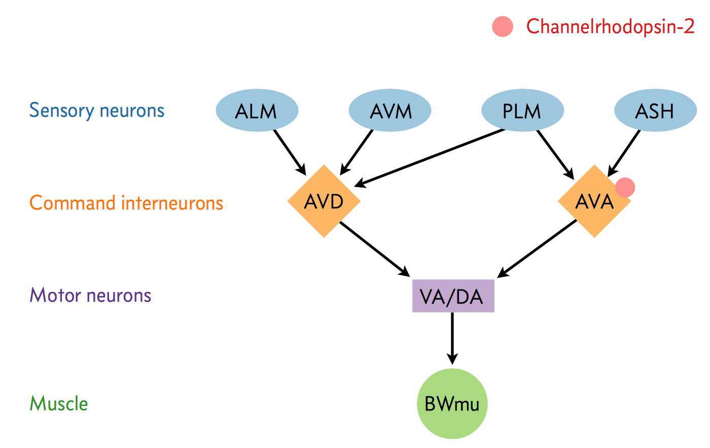
In the experiment, we used optogenetics to dissect the function of individual neurons in this circuit. We worked with two optogenetic worm strains. The ASH strain has channelrhodopsin (ChR2, represented by a red barrel in the figure above) expressed only in the ASH sensory neuron. When we shine blue light on this strain, we should activate the ChR2, which will allow sodium and calcium cations to flow into the neuron, simulating an action potential. We want to quantify how robustly this stimulation will cause the worm to exhibit aversion behavior and reverse.
We also studied an AVA strain that has channelrhodopsin expressed only in the AVA command interneuron. Our goal is to quantify the effects of stimulating this neuron in terms of reversals compared to the ASH neuron and to wild type.
The True/False data here are the whether or not the worms undergo a reversal. Here is what the students observed.
| Strain | Year | Trials | Reversals |
|---|---|---|---|
| WT | 2017 | 55 | 7 |
| ASH | 2017 | 54 | 18 |
| AVA | 2017 | 52 | 28 |
| WT | 2016 | 36 | 6 |
| ASH | 2016 | 35 | 12 |
| AVA | 2016 | 36 | 30 |
| WT | 2015 | 35 | 0 |
| ASH | 2015 | 35 | 9 |
| AVA | 2015 | 36 | 33 |
For the purposes of this problem, assume that we can pool the results from the two years to have 13/126 reversals for wild type, 39/124 reversals for ASH, and 91/124 reversals for AVA.
Our goal is to estimate $p$, the probability of reversal for each strain. That is to say, we want to compute $P(p\mid r, n)$, where $r$ is the number of reversals in $n$ trials.
a) Write down an expression for the posterior probability density function for $P(p\mid r, n)$. That is, write down an expression for the likelihood and prior.
b) Plot the posterior probability density function for each of the three strains. What can you conclude from this?
c) We really want to compare two strains, which we will label 1 and 2 (e.g., "1" could be wild type and "2" could be ASH). So, we would like to compute $P(\delta\mid r_1, r_2, n_1, n_2)$, where $\delta \equiv p_2 - p_1$. Toward that end, write down an expression for $P(p_1, p_2 \mid r_1, r_2, n_1, n_2)$.
d) Perform a change of variables, defining $\delta \equiv p_2 - p_1$ and $\gamma \equiv p_2 + p_1$, to write $P(\gamma, \delta \mid r_1, r_2, n_1, n_2)$. Be sure to indicate for which values of $\delta$ and $\gamma$ that $P(\gamma, \delta \mid r_1, r_2, n_1, n_2)$ is zero.
e) Write down what integral you would have to do to get the marginal distribution $P(\delta\mid r_1, r_2, n_1, n_2)$. You do not need to evaluate the integral, just write it down to demonstrate now nasty it is. You will solve this marginalization problem using Markov chain Monte Carlo in a future problem set.
Problem 3.4: The effects of a prior (10 pts extra credit)
In this problem, we will do a computational exploration of how the choice of prior might affect the posterior. To demonstrate this, we will use the zebrafish sleep data from Tutorial 2a. Our goal is to get a parameter estimate for the number of minutes of sleep for wild type fish on the fifth night. We define a fish to be "asleep" for a minute if the number of seconds of activity in that minute is less than 0.1. First, we will extract that value for all of the wild type fish using the tidying pipeline we developed in Tutorial 2a.
# Load in the genotype file, call it df_gt for genotype DataFrame
df_gt = pd.read_csv('../data/130315_1A_genotypes.txt',
                    delimiter='\t',
                    comment='#',
                    header=[0, 1])

# Rename columns
df_gt.columns = ['wt', 'het', 'mut']

# Melt to tidy
df_gt = pd.melt(df_gt, var_name='genotype', value_name='location').dropna()

# Reset index
df_gt = df_gt.reset_index(drop=True)

# Integer location names
df_gt.loc[:,'location'] = df_gt.loc[:, 'location'].astype(int)

# Read in activity data
df = pd.read_csv('../data/130315_1A_aanat2.csv', comment='#')

# Merge with genotype data
df = pd.merge(df, df_gt)

# Convert time to datetime
df['time'] = pd.to_datetime(df['time'])

# Column for light or dark
df['light'] = (  (df['time'].dt.time >= pd.to_datetime('9:00:00').time())
               & (df['time'].dt.time < pd.to_datetime('23:00:00').time()))

# Indices we want
inds = (  (~df['light'])
        & (df['day'] == 5)
        & (df['activity'] < 0.1)
        & (df['genotype'] == 'wt') )

# Pluck our data and count number of sleeping minutes; store as NumPy array
n_sleep_min = df[inds].groupby('location')['location'].count().values

# Take a look
n_sleep_min
So, we have 17 measurements of the number of sleep minutes on the fifth night of the life of wild type fish. We define these measurements as $\mathbf{x} \equiv [303, 278, \ldots]$ min.
a) Assume that the measurements come from a Gaussian distribution with mean $\mu$ and unknown variance $\sigma$. Write down an expression for the likelihood, $P(\mathbf{x}\mid \mu, \sigma)$.
b) Assuming a uniform prior for $\mu$ and a Jeffreys prior for $\sigma$, plot the posterior as a contour plot in the $\mu$-$\sigma$ plane.
c) Now use a uniform prior for $\sigma$ instead of a Jeffreys prior and repeat the plot. Comment on how big of a difference you see.
d) Now use an informative prior for $\mu$ and a Jeffreys prior for $\sigma$. Specifically, use
\begin{align} P(\mu,\sigma \mid \mu_\mathrm{prior}, \sigma_\mu) \propto \frac{1}{\sigma\,\sigma_\mu}\exp\left[-\frac{(\mu - \mu_\mathrm{prior})^2}{2\sigma_\mu^2}\right]. \end{align}
For this illustration, we will use $\mu_\mathrm{prior} = 200$ minutes and $\sigma_\mu = 100$ minutes. Plot the posterior for this statistical model.
e) The prior in part (d) was weakly informative. Now let's use a more informative prior, taking $\sigma_\mu = 20$ minutes.
f) Comment on how informative the prior is affects your parameter estimates.