BE/Bi 103, Fall 2017: Homework 4¶

Due 1pm, Sunday, October 22¶

This homework was generated from an Jupyter notebook. You can download the notebook here.

Problem 4.1: Dorsal gradients in Drosophila embryos (55 pts)¶

We will use a data set from Angela Stathopoulos's lab, acquired to study morphogen profiles in developing fruit fly embryos. The original paper is Reeves, Trisnadi, et al., Dorsal-ventral gene expression in the Drosophila embryo reflects the dynamics and precision of the Dorsal nuclear gradient, Dev. Cell., 22, 544-557, 2012, and the data set may be downloaded here.

In this experiment, Reeves, Trisnadi, and coworkers measured expression levels of a fusion of Dorsal, a morphogen transcription factor important in determining the dorsal-ventral axis of the developing organism, and Venus, a yellow fluorescent protein along the dorsal/ventral- (DV) coordinate. They put this construct on the third chromosome, while the wild type dorsal is on the second. Instead of the wild type, they had a homozygous dorsal-null mutant on the second chromosome. The Dorsal-Venus construct rescues wild type behavior, so they could use this construct to study Dorsal gradients.

Dorsal shows higher expression on the ventral side of the organism, thus giving a gradient in expression from dorsal to ventral which can be ascertained by the spatial distribution of Venus fluorescence intensity.

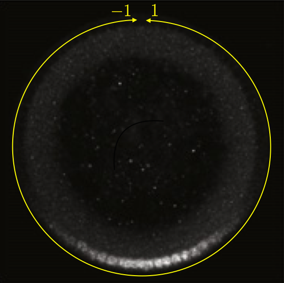
This can be seen in the image below, which is a cross section of a fixed embryo with anti-Dorsal staining. The bottom of the image is the ventral side and the top is the dorsal side of the embryo. The DV coordinate system is defined by the yellow line. It is periodic, going from $-1$ to $1$. The DV-coordinate is therefore defined in relative terms around the embryo and is dimensionless. The ventral nuclei show much higher expression of Dorsal. The image is adapted from the Reeves, Trisnadi, et al. paper.

A quick note on nomenclature: Dorsal (capital D) is the name of the protein product of the gene dorsal (italicized). The dorsal (adjective) side of the embryo is its back. The ventral side is its belly. Dorsal is expressed more strongly on the ventral side of the developing embryo. This can be confusing.

To quantify the gradient, we need a metric for gradient width. Reeves, Trisnadi, and coworkers chose one method of quantifying the gradient, but we will use a different one here. Specifically, we will assume that the fluorescence intensity profile is

\begin{align} F(x;F_\mathrm{bg}, F_0, \lambda, x_0) = F_\mathrm{bg} + F_0\,\mathrm{e}^{-|x-x_0|/\lambda}, \end{align}

where $F(x;F_\mathrm{bg}, F_0, \lambda, x_0)$ is the fluorescence intensity at position $x$. $F_\mathrm{bg}$ is the background fluorescence level, and $F_0$ sets the fluorescence scale. The parameter $x_0$ accounts for possible inaccuracies in setting the origin of the coordinate access system. Namely, it is the location of the peak fluorescence intensity. Finally, we have $\lambda$, which is the parameter we are after to quantify the width of the gradient.

The file reeves_dv_profile_over_time.csv contains the measured level of fluorescence intensity coming from the Dorsal-Venus construct at different stages of development. Timing of development in the Drosophila embryo based on nuclear cycles, the number of nuclear divisions that have happened since fertilization. Prior to cellularization of the syncytium, there are 14 rounds of nuclear division. Reeves, Trisnadi, et al. measured Dorsal-Venus expression at nuclear cycle 11, 12, 13, and 14.

a) We are going to work through a pipeline. Assume the data have already been validated. Now, tidy the data set. (There are many ways you can do this; I did it in at least three different ways. Referring to the Pandas docs might be useful, as usual.)

b) Next is EDA. Explore the data set by making instructive plots.

c) Now it is time for statistical inference. Write down expressions for the likelihood, prior, and posterior for a regression of this sort of data. Be sure to explicitly state which assumptions go into these choices.

d) Perform regressions by optimization to quantify the width of the Dorsal-Venus gradient at each nuclear cycle. (This means that you need to find $\lambda_\mathrm{MAP}$.) Be sure to report error bars on the parameters you obtain. You should also plot the fluorescence intensity profile corresponding to the most probable parameter values along with the experimentally observed data points.

Problem 4.2: HIV clearance and a warning about regressions (45 pts)¶

A human immunodeficiency virus (HIV) is a virus that causes host organisms to develop a weaker, and sometimes ineffective, immune system. HIV inserts its viral RNA into a target cell of the immune system. This virus gets reverse transcribed into DNA and integrated into the host cell's chromosomes. The host cell will then transcribe the integrated DNA into mRNA for the production of viral proteins and produce new HIV. Newly created viruses then exit the cell by budding off from the host. HIV carries the danger of ongoing replication and cell infection without termination or immunological control. Because CD4 T cells, which communicate with other immune cells to activate responses to foreign pathogens, are the targets for viral infection and production, their infection leads to reductions in healthy CD4 T cell production, causing the immune system to weaken. This reduction in the immune response becomes particularly concerning after remaining infected for longer periods of time, leading to acquired immune deficiency syndrome (AIDS).

Perelson and coworkers have developed mathematical models to study HIV populations in the eukaryotic organisms. HIV-1 infects cells at a rate $k$ and is produced from these infected T cells at a rate $p$. On the other hand, the viruses are lost due to clearance by the immune system of drugs, which occurs at a rate $c$, and infected cells die at a rate $\delta$ (Figure from Perelson, Nat. Rev. Immunol., 2, 28-36, 2002)

/Basic model of viral infection

The above process can be written down as a system of differential equations.

\begin{align} \frac{dT^*}{dt} &= k V_I T - \delta T^*\\[1em] \frac{dV_I}{dt} &= -cV_I\\[1em] \frac{dV_{NI}}{dt} &= N \delta T^{*} - c V_{NI}, \end{align}

Here, $T(t)$ is the number of uninfected T-cells at time $t$, and $T^*$ is the number of infected T cells. Furthermore, there is a concentration $V_I(t)$ of infectious viruses that infect T cells at the rate $k$. We also have a concentration $V_{NI}$ of innocuous viruses. We define $N(t)$ to be the number of newly produced viruses from one infected cell over this cell's lifetime. We can measure the total viral load, $V(t) = V_I(t) + V_{NI}(t)$. If we initially have a viral load of $V(0) = V_0$, we can solve the system of differential equations to give

\begin{align} V(t) = V_0e^{-ct} + \frac{cV_0}{c-\delta}\left[\frac{c}{c-\delta}(e^{-{\delta}t} - e^{-ct}) - {\delta}te^{-ct}\right]. \end{align}

We will take viral load data from a real patient (which you can download here) and perform a regression to evaluate the parameters $c$ and $\delta$. The patient was treated with the drug Ritonavir, a protease inhibitor that serves to clear the viruses; i.e., it modulates $c$. So, in the context of the model, $c$ is a good parameter to use to understand the efficacy of a drug.

a) Perform a regression on these data using the theoretical temporal curve for the viral load. That is, obtain estimates for $V_0$, $c$, and $\delta$ by finding the MAP and computing error bars.

b) Plot the posterior distribution over the interval $0 \le \delta, c \le 10$ days$^{-1}$. Does this plot raise any serious issues about how you estimate $c$ and $d$? What experiments might you propose to help deal with these problems? Hint: In order to compute the marginalized posterior,

\begin{align} g(c, \delta \mid D) = \int_0^\infty \mathrm{d}V_0 \,g(c, \delta, V_0 \mid D, I), \end{align}

you can perform numerical quadrature using functions like np.trapz(). If you are having trouble doing that, make a plot of $g(c, \delta, V_0 \mid D)$ in the $c$-$\delta$ plane with $V_0$ fixed at its most probable value.

Problem 4.3: Checking model assumptions (10 pts extra credit)¶

In Tutorial 4a, we did a check on some of the model assumptions, in particular that $Vs/V_0 \ll 1$ and that the aspect ratio $k$ is the same for all spindles. Based on the analysis in that tutorial, are you concerned that a nonconstant $k$ might affect your analysis? Implement a remedy for the potential effects. As a reminder, the data set may be downloaded here.