Tutorial 8b: Extracting data from images
(c) 2017 Justin Bois. This work is licensed under a Creative Commons Attribution License CC-BY 4.0. All code contained herein is licensed under an MIT license.
This exercise was generated from a Jupyter notebook. You can download the notebook here.
import glob
import os
import numpy as np
import pandas as pd
import scipy.signal
# Image processing tools
import skimage
import skimage.io
import bebi103
import bokeh
bokeh.io.output_notebook()
Before we can start working with images, we need to know how to do all of the more mundane things with them, like organizing, loading, storing, etc. Images that you want to analyze come in all sorts of formats and are organized in many different ways. One instrument may give you a TIFF stack consisting of 8-bit images. Another may give you a directory with lots of images in it with different names. And so many instruments give you data in some proprietary format. You need to know how to deal with lots of file formats and organization.
In this course, we will analyze various images, including microscopy images. I generally will give them to you in exactly the format I received them in.
In today's tutorial, we will use a data set from three alumni of this class (Mike Abrams, Claire Bedbrook, and Ravi Nath) to practice loading images, defining ROIs, and some basic skills for extracting information from images. The findings from this research were published here. You can download the data set here.
In this tutorial and throughout the class, we will use scikit-image to do almost all of our image processing. It has continual development, with new features constantly being added. For the fairly simple image processing we'll do in this course, it suffices for most of what we need. The course website has links to many other image processing toolkits, some Python-based and many not.
The data set
The data set comes from three Caltech graduate students, Mike Abrams, Claire Bedbrook, and Ravi Nath, who studied day and night behavior in jellyfish. They photographed jellyfish over time and studied their pulsing behavior. You can download a movie of pulsing jellyfish here. A typical image is shown below.
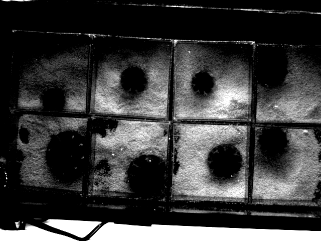
A single jellyfish lives in each box. The boxes are 4 by 4 inches. The jellyfish constantly contract and relax in a pulsing motion. Our task in this tutorial is to get traces so we can measure pulse frequency.
We have two different data sets, day and night, each contained in their own directory. Each image they acquired is stored as a TIFF image. The frame rate was 15 frames per second.
Let's take a look at the structure of the directory with the images. We will use the glob module, which allows us to specify string with wild cards to specify files of interest.
# The directory containing daytime data
data_dir = '../data/Cassiopea_Pulsation/day'
# Glob string for images
im_glob = os.path.join(data_dir, '*.TIF')
# Get list of files in directory
im_list = glob.glob(im_glob)
# Let's look at the first 10 entries
im_list[:10]
We see that the images are nicely named so that successive frames are stored in order. This is convenient, and when this is not the case, you should rename files so that when listed in alphabetical order, they also appear in temporal order.
Loading and displaying images
The workhorse for much of our image processing is scikit-image. We will load our first image using scikit-image. When importing scikit-image, it is called skimage, and we need to import the submodules individually. The submodule for reading and writing images is skimage.io. We can use it to load and display an image. Let's start with the first jellyfish image.
# Read in the image using skimage
im = skimage.io.imread(im_list[0])
# Let's get information about the image
print(type(im), im.dtype, im.shape)
So, the image is stored as a NumPy array of 16-bit ints. The array is 3$\times$480$\times$640, which means this is an RGB image. The first index of the image indicates the channel (red, green, or blue). Cameras often store black and white images as RGB, so let's see if all three channels are the same.
# Test to see if each R, G, and B value is the same
((im[:,:,0] == im[:,:,1]) & (im[:,:,1] == im[:,:,2])).all()
Indeed they are, so we can just consider one of the channels in our analysis.
# Just slice the red channel
im = im[:,:,0]
Now, let's use bokeh to take a look at the image.
p = bebi103.viz.imshow(im)
bokeh.io.show(p)
Setting the scale
Remember, scientific images are not just pretty pictures. It is crucially important that you know the interpixel distance and that the images have a scale bar when displayed (or better yet, have properly scaled axes, like we have in Bokeh plots).
For some microscope set-ups, we already know the physical length corresponding to the interpixel distance. We often take a picture of something with known dimension (such as a stage micrometer) to find the interpixel distance. In the case of these jellyfish images, we know the boxes are 4$\times$4 inches. We can get the locations of the boxes in units of pixels by clicking on the image and recording the positions of the clicks.
We can use the record_clicks kwarg of the bebi103.viz.imshow() function to get the click positions in a copy-able format for use in a NumPy array.
p = bebi103.viz.imshow(im, record_clicks=True)
bokeh.io.show(p)
I can now copy the coordinates to make a NumPy array.
xy = np.array([[348.2218, 243.6252],[500.1257, 239.2508],])
We can use these points to compute the length of a side of a box.
box_length = np.sqrt((xy[1][1] - xy[0][1])**2 + (xy[1][0] - xy[0][0])**2)
The interpixel distance is then 4 inches / box_length. We will compute it in centimeters.
interpixel_distance = 4 / box_length * 2.54
Now that we know the interpixel distance, we can display the image with appropriate scaling of axes.
p = bebi103.viz.imshow(im,
interpixel_distance=interpixel_distance,
length_units='cm')
bokeh.io.show(p)
Loading a stack of images
While we have done some nice things with single images, we really want to be able to sequentially look at all of the images of the movie, a.k.a. the stack of images.
scikit-image has a convenient way to do this using the skimage.io.ImageCollection class. We simple give it a string matching the pattern of the file names we want to load. In our case, this is im_glob that we have already defined. An important kwarg is conserve_memory. If there are many images, it is best to select this to be True. For few images, selecting this to be False will result in better performance because all of the images will be read into RAM. Let's load the daytime movie as an ImageCollection. (Note: we're not actually loading them all in; we just creating an object that knows where the images are so we can access them at will.)
ic = skimage.io.ImageCollection(im_glob, conserve_memory=True)
Conveniently, the ImageCollection has nice properties. Typing len(ic) tells how many images are in the collection. ic[157] is the 157th image in the collection. There is one problem, though. All of the images are read in with all three channels. We would like to only include one channel, since the others are redundant. To do this, we can instantiate the ImageCollection with the load_func kwarg. This specifies a function that reads in and returns a NumPy array with the image. The default is load_func=skimage.io.imread, but we can write out own. We'll write a function that loads the image and then just returns the red channel and reinstantiate the ImageCollection using that load function.
def squish_rgb(fname, **kwargs):
"""
Only take one channel. (Need to explicitly have the **kwargs to play
nicely with skimage.io.ImageCollection.)
"""
im = skimage.io.imread(fname)
return im[:,:,0]
ic = skimage.io.ImageCollection(im_glob,
conserve_memory=True,
load_func=squish_rgb)
We should also have time stamps for the data in the images. We know the frame rate is 15 frames per second, so we can attach times to each image. Normally, these would be in the metadata of the images and we would fish that out, but for this example, we will just generate our own time points (in units of seconds).
fps = 15
t = np.arange(0, len(ic)) / fps
Setting an ROI
A region of interest, or ROI, is part of an image or image stack that we would like to study, ignoring the rest. Depending on the images we are analyzing, we may be able to automatically detect ROIs based on well-defined criteria. Often, though, we need to manually pick regions in an image as our ROI.
scikit-image is an open source project that is constantly under development. It currently does not have a way to specify ROIs, but it is on the list of functionality to be added.
So, I wrote my own ROI utility, which is included in bebi103.image submodule. It takes a set of vertices that define a polygon, the inside of which constitutes a region of interest. (Note that the polygon cannot have crossing lines.) It returns a tuple that contains a mask for the ROI, a bounding box, and the mask for an image consisting entirely of the bounding box. An ROI mask is the same shape as the image, except where the image has a pixel value, the ROI mask has a True value if the pixel is within the ROI and has a False value it if is outside. The bounding box defines the smallest square subimage that completely contains the ROI. Finally, it is convenient to have a mask that is reindexed such that (0,0) is the upper left corner of the bounding box.
To get the vertices, we can again use the bebi103.viz.imshow() function with the record_clicks=True kwarg. When you do this, though, make sure the image is displayed in units of pixels, since the ROI is determined in units of pixels. Secondly, use the flip=False kwarg. This is necessary because matrix indices start in the upper left corner, and not the lower left corner like plots. Remember that an image is stored as a Numpy array. In this example, I clicked a square in the image to select a single box.
bokeh.io.show(bebi103.viz.imshow(im, flip=False, record_clicks=True))
I can paste the results of my clicks into a Numpy array, and then use them to get the ROI.
# I clicked the image to get these coordinates for vertices
verts = np.array([[346.0797, 243.6736],
[491.1287, 249.2246],
[486.8203, 392.1627],
[343.2075, 385.9178]])
Now we can use bebi103.image.verts_to_roi() to make make the ROI.
roi, roi_bbox, roi_box = bebi103.image.verts_to_roi(verts, *ic[0].shape)
Now that we have defined the ROI, let's look at it. We will use a trick where we take a grayscale image, convert it to RGB, and then add more blue in certain regions to highlight.
# Make grayscale image that is now RGB
im = np.dstack(3*[skimage.img_as_float(ic[0])])
# Max out blue channel
im[roi, 2] = skimage.dtype_limits(im)[1]
# Look at the image
p = bebi103.viz.imshow(im, color_mapper='rgb')
bokeh.io.show(p)
If you just want to look at the region of the image that bounds the ROI, you can do the following.
# Get cropped image and ROI within it
im = ic[0][roi_bbox]
im_cropped_roi = roi_box
# Make grayscale image that is now RGB
im = np.dstack(3*[skimage.img_as_float(im)])
# Max out blue channel
im[im_cropped_roi,2] = skimage.dtype_limits(im)[1]
# Look at the image
p = bebi103.viz.imshow(im, color_mapper='rgb')
bokeh.io.show(p)
So, when working with ROIs, the roi, roi_bbox, and roi_box are useful tools to automatically index the original image to get what you are interested in. We could also modify our load_func() for our ImageCollection to just load in an ROI.
# Define load_func that only gives region bounding ROI
def load_roi(fname, roi_bbox=None, **kwargs):
"""
Image loading function to only load ROI.
"""
if roi_bbox is None:
return skimage.io.imread(fname)[:,:,0]
else:
return skimage.io.imread(fname)[:,:,0][roi_bbox]
# Load image collection
ic = skimage.io.ImageCollection(im_glob, conserve_memory=True,
load_func=load_roi, roi_bbox=roi_bbox)
# Look at first image
p = bebi103.viz.imshow(ic[0])
bokeh.io.show(p)
Some simple analysis
We are interested in the rate at which the jellyfish pulse. Since the jellyfish are dark on a black background, we could just watch how the total pixel intensity of our respective ROIs change over time to get the pulsing frequency. This will not really tell us about the shape of the jellyfish or any fine detail, but it will hopefully be enough to get us an estimate of pulsing frequency.
To be more concrete, our goal is to find the distribution of inter-contraction times. If the distribution is tightly peaked, we have periodic pulsing and we can estimate a frequency. Otherwise, we might notice pause events that we can see qualitatively in the movies.
We will analyze the jellyfish in our current ROI. To start with, we'll just compute the total pixel intensity through time.
# Set up NumPy array to store total pixel intensity
total_int = np.empty(len(t))
# Look through and compute total intensity in the ROI
for i, im in enumerate(ic):
total_int[i] = ic[i][roi_box].sum()
Let's plot the result!
p = bokeh.plotting.figure(plot_width=650,
plot_height=300,
x_axis_label='time (s)',
y_axis_label='total intensity')
p.line(t, total_int, line_width=2, line_join='bevel')
bokeh.io.show(p)
Since the intensity units are arbitrary, we can let's subtract the mean and rescale the data so they go from -1 to 1.
total_int -= total_int.mean()
total_int = 1 + 2 * ((total_int - total_int.max())
/ (total_int.max() - total_int.min()))
p = bokeh.plotting.figure(plot_width=650,
plot_height=300,
x_axis_label='time (s)',
y_axis_label='total intensity')
p.line(t, total_int, line_width=2, line_join='bevel')
bokeh.io.show(p)
Your turn
If you zoom in on the signal, you will see peaks and valley, corresponding to contractions and relaxations, respectively. Can you use the time series analysis tools from the previous tutorial to get the interpulse times?
Can you do the similar analysis with the night time data set and compare the results to the day? Can you do it for all eight jellyfish? Can you analyze the time series to get the inter-peak intervals? What do you observe? This is actually one of your homework problems.