BE/Bi 103, Fall 2017: Homework 6
Due 1pm or 7pm, Sunday, November 11
(c) 2018 Justin Bois. With the exception of pasted graphics, where the source is noted, this work is licensed under a Creative Commons Attribution License CC-BY 4.0. All code contained herein is licensed under an MIT license.
This document was prepared at Caltech with financial support from the Donna and Benjamin M. Rosen Bioengineering Center.

This homework was generated from an Jupyter notebook. You can download the notebook here.
Problem 6.1: Modeling and parameter estimation for Boolean data (40 pts)
In this problem, we will work with data of the True/False type. Lots of data sets in the biological sciences are like this. For example, we might look at a certain mutation in Drosophila that affects development and we might check whether or not eggs hatch.
The data we will use comes from an experiment we have done for the last few years in Bi 1x here at Caltech. The experiment was developed by Meaghan Sullivan. We studied a neural circuit in C. elegans using optogenetics.
A neural circuit is a series of interconnected neurons that create a pathway to transmit a signal from where it is received to where it causes a behavioral response in an animal. An example is the neural circuit involved in reversals in C. elegans. This circuit consists of three types of neurons: sensory neurons receive stimuli from the environment, command interneurons integrate information from many sensory neurons and pass a signal to the motor neurons, and motor neurons that control worm behavior, such as reversals.
There are six non-motor neurons acting in a circuit that responds to environmental cues and triggers a reversal, a shown in the figure below (based on Schultheis et. al. 2011). These include four sensory neurons (ALM, AVM, ASH, and PLM) and two interneurons (AVD and AVA). Each sensory neuron is sensitive to a different type of stimulus. For example, the sensory neuron we are studying (ASH) is sensitive to chemosensory stimuli such as toxins, while another neuron (PLM) is sensitive to mechanical stimuli (touch) in the posterior part of the worm's body. The sensory neurons send signals that are integrated by the two command interneurons (AVA and AVD). Each sensory neuron can provide an impulse to the command interneurons at any time. In order for the command interneuron to fire and activate motor neurons, the sum of the stimuli at any point in time must exceed a certain threshold. Once the stimuli from one or more sensory neurons has induced an action potential in a command interneuron, that signal is passed to motor neurons which will modulate worm behavior.
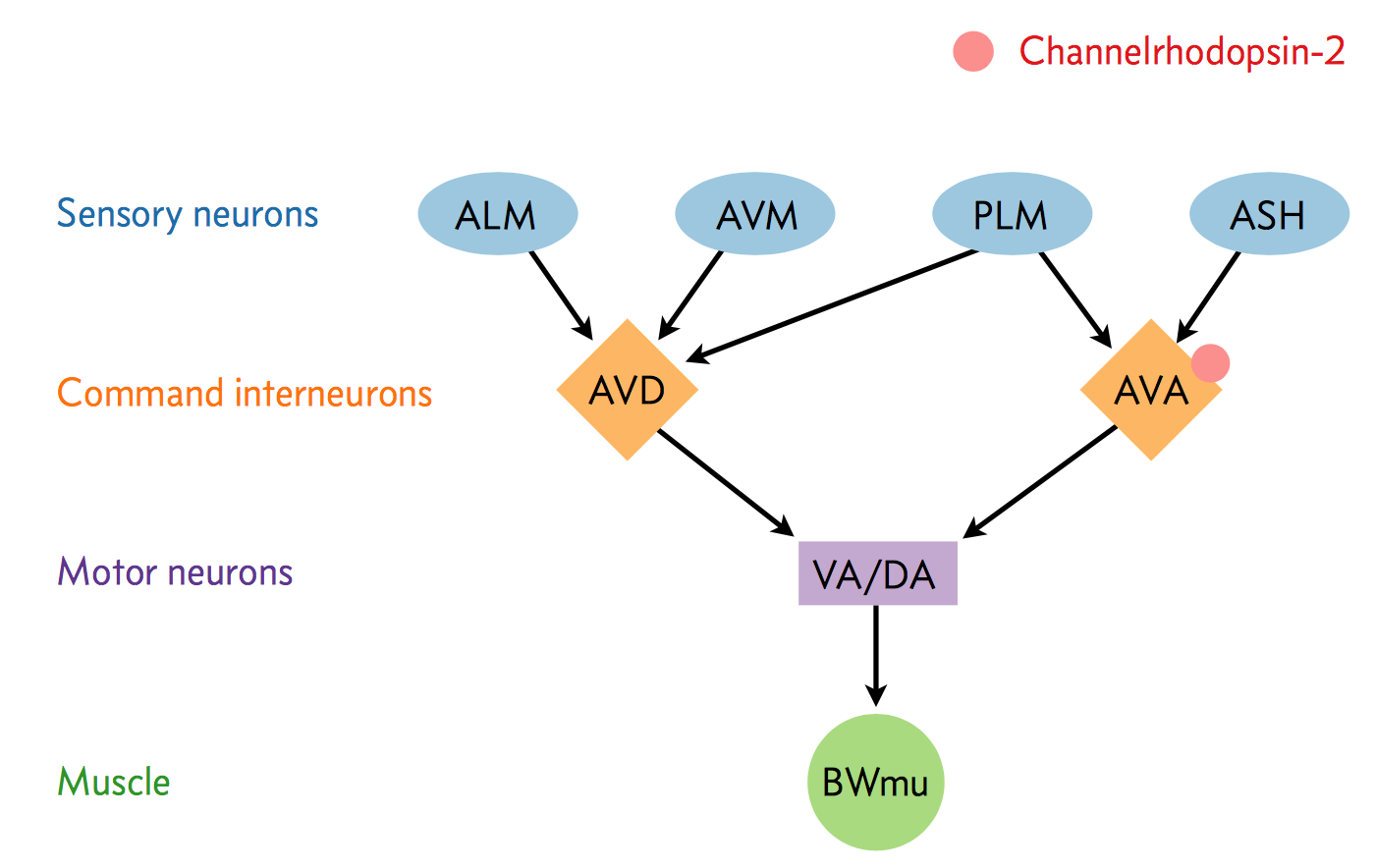
In the experiment, we used optogenetics to dissect the function of individual neurons in this circuit. We worked with two optogenetic worm strains. The ASH strain has channelrhodopsin (ChR2, represented by a red barrel in the figure above) expressed only in the ASH sensory neuron. When we shine blue light on this strain, we should activate the ChR2, which will allow sodium and calcium cations to flow into the neuron, simulating an action potential. We want to quantify how robustly this stimulation will cause the worm to exhibit aversion behavior and reverse.
We also studied an AVA strain that has channelrhodopsin expressed only in the AVA command interneuron. Our goal is to quantify the effects of stimulating this neuron in terms of reversals compared to the ASH neuron and to wild type.
The True/False data here are the whether or not the worms undergo a reversal. Here is what the students observed.
| Strain | Year | Trials | Reversals |
|---|---|---|---|
| WT | 2017 | 55 | 7 |
| ASH | 2017 | 54 | 18 |
| AVA | 2017 | 52 | 28 |
| WT | 2016 | 36 | 6 |
| ASH | 2016 | 35 | 12 |
| AVA | 2016 | 36 | 30 |
| WT | 2015 | 35 | 0 |
| ASH | 2015 | 35 | 9 |
| AVA | 2015 | 36 | 33 |
For the purposes of this problem, assume that we can pool the results from the three years to have 13/126 reversals for wild type, 39/124 reversals for ASH, and 91/124 reversals for AVA.
Our goal is to estimate $\theta$, the probability of reversal for each strain. That is to say, we want to compute $g(\theta\mid n, N)$, where $n$ is the number of reversals in $N$ trials.
a) Develop a generative model (that is, specify the joint distribution $\pi(n, \theta\mid N) = f(n\mid \theta, N)\,g(\theta)$) for the observed reversals. Be sure to do prior predictive checks and justify why you chose the model you did. Biological hint: C. elegans have no mode of sensing light at all. So, a wild type worm without and Channelrhodopsin has no means of detecting light. Modeling hint: The Beta distribution is very useful for modeling probabilities of probabilities, like θ in this problem.
b) Plot the posterior probability density function for each of the three strains. What can you conclude from this?
Problem 6.2: Least squares (20 pts)
You may have heard that to estimate the best-fit parameters for a regression, you should "minimize the sum of the squares of the residuals." In this problem, we will parse what that means and understand it in the context of generative Bayesian modeling.
Say I have some (x, y) data, where x is the independent variable (known essentially exactly; this could be something like time) and y is the dependent variable (which has some stochasticity of noise in its measurement). Imagine that we have derived a theoretical relation between our expected y and x, and that relation is written as $y = f_y(x;\theta)$, there $\theta$ is some set of parameters that we wish to determine from our regression.
Our data set is $\{(x_1, y_1), (x_2, y_2), \ldots, (x_N, y_N)\}$. We assume the measurements of $y$ are i.i.d. and Gaussian distributed.
\begin{align} y_i \sim \mathrm{Norm}(f_y(x_i;\theta), \sigma_i) \;\;\forall i. \end{align}
A residual for a data point is defined as
\begin{align} r_i = \frac{y_i - f_y(x_i;\theta)}{\sigma_i}. \end{align}
The sum of the squares of the residuals is then
\begin{align} \sum_{i=1}^N r_i^2 = \sum_{i=1}^N\,\frac{(y_i - f_y(x_i;\theta))^2}{\sigma_i^2}. \end{align}
a) Show that finding the parameters $\theta$ that minimize the sum of the squares of the residuals is equivalent to finding the MAP parameters for a model with the above likelihood and Uniform priors on all parameters. Note that the values of $\sigma_i$ are usually known when taking this approach; they are not parameters to be estimated.
b) Show further that if we assume homoscedastic errors, that is that $\sigma_i = \sigma$ for all $i$, then we do not need to consider the parameter $\sigma$ at all in finding the MAP values for $\theta$. The assumption of homoscedasticity is often made when the $\sigma_i$ are not known. This is often the procedure that is done with least sqaures regression.
c) Discuss any issues you see with taking this approach. Think generatively.
Problem 6.3: Analysis of FRAP data (40 pts)
In homework set 4), we began analyzing a FRAP experiment by Nate Goehring and corworkers. You performed image analysis to obtain the mean fluorescence of the bleach spot versus time. In this problem, you will use those data to obtain estimates for the diffusion coefficient $D$ and chemical rate constant $k_\mathrm{off}$ for the PH-PLCd1/PIP2 complex.
As a reminder, we are taking a simplified approach, but there is more sophisticated analysis we can do to get better estimates for the phenomenological coefficients. These are discussed in the Goehring, et al. paper. Instead, we will use the the mean fluorescence of the bleached region, $I(t)$ to perform our analysis. As derived in their paper,
\begin{align} I_\mathrm{norm}(t) \equiv I(t)/I_0 &= f_f\left(1 - f_b\,\frac{4 \mathrm{e}^{-k_\mathrm{off}t}}{d_x d_y}\,\psi_x(t)\,\psi_y(t)\right),\\[1mm] \text{where } \psi_i(t) &= \frac{d_i}{2}\,\mathrm{erf}\left(\frac{d_i}{\sqrt{4Dt}}\right) -\sqrt{\frac{D t}{\pi}}\left(1 - \mathrm{e}^{-d_i^2/4Dt}\right), \end{align}
where $d_x$ and $d_y$ are the extent of the photobleached box in the $x$- and $y$-directions, $f_b$ is the fraction of fluorophores that were bleached, $f_f$ is the fraction of total fluorescent species left after photobleaching, and $\mathrm{erf}(x)$ is the error function. Here, $I_0$ is the mean fluorescence in the bleach spot before bleaching. Note that this function is defined such that the photobleaching event occurs at time $t = 0$.
Your task in this problem is to develop a generative model and then to find estimates for the parameters of the model. We will revisit this problem again later in the course and build a hierarchical model. For this problem, consider each of the eight trials separately and use optimization to find the MAP parameter values for each trial and make a Gaussian approximation of the posterior to give an approximate 95% credible region.
You should have acquired a data set of mean fluorescence versus time, and you should use that for your analysis. If you do not have that data set, you can download those generated in the solutions here.