Tutorial 6a: Model generation and prior predictive checks
(c) 2018 Justin Bois. With the exception of pasted graphics, where the source is noted, this work is licensed under a Creative Commons Attribution License CC-BY 4.0. All code contained herein is licensed under an MIT license.
This document was prepared at Caltech with financial support from the Donna and Benjamin M. Rosen Bioengineering Center.

This tutorial was generated from an Jupyter notebook. You can download the notebook here.
import numpy as np
import pandas as pd
import scipy.special
import scipy.stats as st

import bebi103

import altair as alt
import bokeh.io
bokeh.io.output_notebook()
When we do generative modeling, it is important to understand what kind of data might be generated from our model before looking at the data. In this tutorial, we discuss how we can come up with a generative Bayesian model, that is specifying the prior and likelihood, and then checking to make sure it makes sense and can actually generate reasonable data sets.
Building a generative model
When considering how to build the model, we should think about the data generation process. We generally specify the likelihood first, and then use it to identify what the parameters are, which tells us what we need to specify for the prior. Indeed, the prior can often only be understood in the context of the likelihood.
Note, though, that the split between the likelihood and prior need even be explicity. When we study hierarchical models, we will see that it is not obvious how to unambiguously define the likelihood and prior. Rather, in order to do Bayesian inference, we really only need to specify the joint distribution, $\pi(y,\theta)$, which is the product of the likelihood and prior.
\begin{align} g(\theta \mid y) = \frac{f(y\mid \theta)\,g(\theta)}{f(\theta)} = \frac{\pi(y, \theta)}{f(\theta)}. \end{align}
After defining the joint distribution, either by defining a likelihood and a prior separately (which is what we usually do) or by directly defining the joint, we should check to make sure that making draws out of it give reasonable results. In other words, we need to ask if the data generation process we have prescribed actually produces data that obeys physical constraints and matches our intuition. The procedure of prior predictive checks enables this. We use the joint distribution to generate parameter sets and data sets and then check if the results make sense. We will learn about doing this using both Numpy and Stan in this tutorial.
The data set
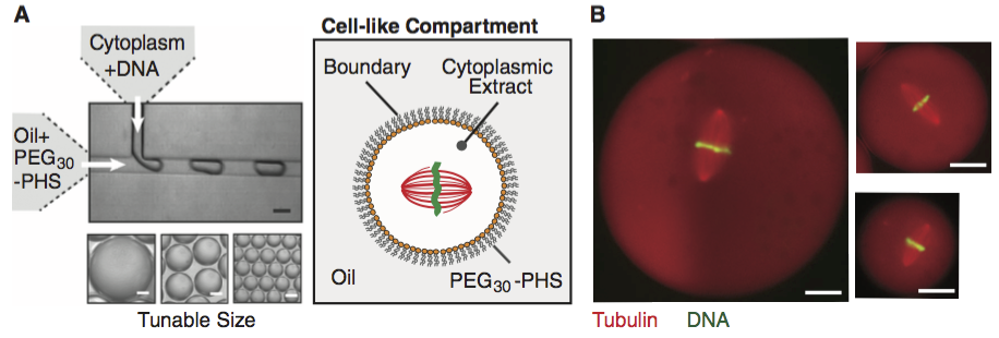
The data set we will use for this analysis comes from Good, et al., Cytoplasmic volume modulates spindle size during embryogenesis Science, 342, 856-860, 2013. You can download the data set here. In this work, Matt Good and coworkers developed a microfluidic device where they could create droplets cytoplasm extracted from Xenopus eggs and embryos (see figure below; scale bar 20 µm). A remarkable property about Xenopus extract is that mitotic spindles spontaneously form; the extracted cytoplasm has all the ingredients to form them. This makes it an excellent model system for studying spindles. With their device, Good and his colleagues were able to study how the size of the cell affects the dimensions of the mitotic spindle; a simple, yet beautiful, question. The experiment is conceptually simple; they made the droplets and then measured their dimensions and the dimensions of the spindles using microscope images. In this tutorial, we will build generative models for the data set, which consists of spindle length-droplet diameter pairs, $(l_i, d_i)$.
We will go ahead and load in the data set so we have it going forward.
df = pd.read_csv('../data/good_invitro_droplet_data.csv', comment='#')

print('N =', len(df))
As we can see, the data set consists of 670 measurements. When we generate our prior predictive data sets, we will generate 670 points.
Model 1: Spindle size is independent of droplet size
As a first model, we propose that the size of a mitotic spindle is inherent to the spindle itself. This means that the size of the spindle is independent of the size of the droplet or cell in which it resides. This would be the case, for example, if construction of the spindle involves length-sensing molecules, such as depolymerizing motor proteins. We define that set length as $\phi$.
The likelihood
Not all spindles will be measured to be exactly $\phi$ µm in length. Rather, there may be some variation about $\phi$ due to natural variation and measurement error. So, we would expect measured length of spindle i to be
\begin{align} l_i = \phi + e_i, \end{align}
where $e_i$ is the noise component of the $i$the datum.
So, we have a theoretical model for spindle length, $l = \phi$, and to get a fully generative model, we need to model the errors $e_i$. A reasonable model assumes
- Each measured spindle's length is independent of all others.
- The variability in measured spindle length is Gaussian.
With these assumptions, we can write the probability density function for $l_i$ as
\begin{align} f(l_i \mid \phi, \sigma) = \frac{1}{\sqrt{2\pi \sigma^2}}\,\exp\left[-\frac{(l_i - \phi)^2}{2\sigma^2}\right]. \end{align}
Since each measurement is independent, we can write the likelihood of the entire data set, which we will define as $l = \{l_1, l_2,\ldots\}$, consisting of $n$ total measurements.
\begin{align} f(l \mid \phi, \sigma) = \prod_{i\in D} f(l_i \mid \phi, \sigma) = \frac{1}{(2\pi \sigma^2)^{n/2}}\,\exp\left[-\frac{1}{2\sigma^2}\sum_{i\in D}(l_i - \phi)^2\right]. \end{align}
We can write this more succinctly, and perhaps more intuitively, as
\begin{align} l_i \sim \text{Norm}(\phi, \sigma) \;\;\forall i. \end{align}
We will generally write our models in this format, which is easier to parse and understand. It also looks similar to a Stan specification, as we will soon see.
Note that in writing this generative model, we have necessarily introduced another parameter, σ, the standard deviation parametrizing the Gaussian distribution. So, we have two parameters in our model, $\phi$ and $\sigma$.
The prior
With our likelihood specified, we need to give a prior for $\phi$ and $\sigma$, $g(\phi, \sigma)$. We will assume that $\phi$ and $\sigma$ are independent; that is, $g(\phi, \sigma) = g(\phi)\,g(\sigma)$. So, we need to specify separate priors for $\phi$ and $\sigma$.
Let's start with $\phi$. We ask, "How big are spindles?" and perform an order-of-magnitude estimate to establish the prior. I think a mitotic spindle should be somewhere around 20 µm. Certainly no smaller than 1 µm, and probably not bigger than 100 µm, which is the on the large end of a typical size of a eukaryotic cell. (I know it sounds strange to say typically size of a eukaryotic cell, since they come in some many varieties, but 30 µm seems like a good upper limit to me.) I'm pretty uncertain, though, so I should not assign a sharp distribution. So, a broad distribution centered at $\phi = 20$ µm will suffice.
\begin{align} \phi \sim \text{Norm}(20, 20). \end{align}
Next, let's try $\sigma$. How much do we expect the spindle length to vary? I would think that 20% variation seems reasonable, but it could be more or less. So, I will again choose a broad distribution centered at $\sigma = 4$ µm.
\begin{align} \sigma \sim \text{Norm}(4, 5). \end{align}
So, we now have a complete model; the likelihood and prior, and therefore the joint distribution, are specified. Here is is (all units are µm):
\begin{align} &\phi \sim \text{Norm}(20, 20), \\[1em] &\sigma \sim \text{Norm}(4, 5), \\[1em] &l_i \sim \text{Norm}(\phi, \sigma) \;\;\forall i. \end{align}
The measurements of the droplet diameters $d_i$ are irrelevant under this model.
If we look at the model with a critical eye, we can immediately see that it has a problem. It is possible that parameters $\phi$ and $\sigma$ could be nonpositive, as could the length, $l_i$. This is impossible in the case of $\sigma$ and unphysical in the cases of $\phi$ and $l_i$. So, these really should be truncated distributions.
That said, it is generally a bad idea to truncate distributions (except and points where their derivatives vanish, like for the Half Normal distribution) when building models. It's both unrealistic and results in more difficult posterior sampling, which ultimately is what we need to do when doing statistical inference.
We will therefore jettison this model out of hand and develop a model that is closer to being physically reasonable. We will keep the same likelihood, since its tails should decay away fast enough to prevent negative values of $l_i$. We instead focus on the prior.
Prior, take 2
Let's start with $\sigma$. It is possible that the spindle size is very carefully controlled. It is also possible that it could be highly variable. So, we can choose a Half Normal prior for $\sigma$ with a large standard deviation. It looks something like this.
sigma = np.linspace(0, 40, 200)
p = bokeh.plotting.figure(width=300, height=200,
                          x_axis_label='σ (µm)',
                          y_axis_label='g(σ)')
p.line(sigma, st.halfnorm.pdf(sigma, 0, 10), line_width=2)
bokeh.io.show(p)
For $\phi$, we can instead take a Log-Normal distribution, with a median of 20 µm. That looks like this.
phi = np.linspace(0, 80, 200)
p = bokeh.plotting.figure(width=300, height=200,
                          x_axis_label='φ (µm)',
                          y_axis_label='g(φ)')
p.line(phi, st.lognorm.pdf(phi, 0.75, loc=0, scale=20), line_width=2)
bokeh.io.show(p)
So, we have an updated model.
\begin{align} &\phi \sim \text{LogNorm}(\ln 20, 0.75),\\[1em] &\sigma \sim \text{HalfNorm}(0, 10),\\[1em] &l_i \sim \text{Norm}(\phi, \sigma) \;\forall i. \end{align}
Note that we should have written $\sigma\sim\text{HalfNorm}(0, 10\,\mu\text{m})$, and to be dimensionally correct, the parameters for the Log-Normal prior on $\phi$ are more correctly written respectively as $\ln(20\,\mu\text{m}/1\,\mu\text{m})$ and $\ln(\mathrm{e}^{0.75\,\mu\text{m}/1\,\mu\text{m}})$. We will however use the shorthand above with the assumption that we are properly taking into account units when defining distributions, and will do so throughout the course.
Prior predictive checks
Let us now generate samples out of this generative model. This procedure is known as prior predictive checking. We first generate parameter values drawing out of the prior distributions for $\phi$ and $\sigma$. We then use those parameter values to generate a data set using the likelihood. We repeat this over and over again to see what kind of data sets we might expect out of our generative model. We can do this efficiently using Numpy's random number generators.
n_ppc_samples = 1000

# Draw parameters out of the prior
phi = np.random.lognormal(np.log(20), 0.75, size=n_ppc_samples)
sigma = np.abs(np.random.normal(0, 10, size=n_ppc_samples))

# Draw data sets out of the likelihood for each set of prior params
ell = np.array([np.random.normal(ph, sig, size=len(df))
                        for ph, sig in zip(phi, sigma)])
There are many ways we could visualize the results. One informative plot is to make an ECDF of each of the data sets. We will thin them out a bit, taking only every 10th data set, to keep the file size of the plot down.
p = bebi103.viz.ecdf(ell[0],
                     x_axis_label='spindle length (µm)',
                     alpha=0.01,
                     line_alpha=0)
for ell_vals in ell[9::10]:
    p = bebi103.viz.ecdf(ell_vals, alpha=0.02, p=p, line_alpha=0)

bokeh.io.show(p)
This looks reasonable, except for the occasional negative spindle lengths. We can check to see how many there are.
Another option is to plot percentiles of the ECDFs. We can do this using the bebi103.viz.predictive_ecdf() function. It expects a data frame that is the same format as exported by Stan, so we need to convert our samples into that format.
data = np.hstack((np.expand_dims(phi, 1), np.expand_dims(sigma, 1), ell))
columns = ['phi', 'sigma'] + [f'ell[{i+1}]' for i in range(len(ell[0]))]

# Make data frame to match output of Stan
df_ppc = pd.DataFrame(data=data, columns=columns)
df_ppc['warmup'] = 0
df_ppc['chain'] = 0
df_ppc['chain_idx'] = np.arange(1, n_ppc_samples+1)

# Take a look, also to show the format of Stan output
df_ppc.head()
We can now use this data frame to make the percentile ECDF plot.
bokeh.io.show(
    bebi103.viz.predictive_ecdf(df_ppc,
                                'ell',
                                x_axis_label='spindle length (µm)'))
In this plot, the median ECDF is shown in the middle, and the colors going out from the median contain the middle 20th, 40th, 60th, and 80th precentiles. The extent of the ECDF gives an indication of the extreme values in the prior predictive data set. The bulk of the spindle lengths lie in a reasonable region, somewhere between zero and 30 µm.
We may be willing to tolerate the negative spindle length values in our model, since any data set, containing no negative values, could easily tug the posterior into positive spindle lengths. Nonetheless, let's check how many negative spindle lengths we get from our generative model. We will compute the fraction of spindle lengths that are negative from our generative model for each of the 1000 data sets we generated and then plot the results as an ECDF.
p = bebi103.viz.ecdf((ell < 0).sum(axis=1) / len(df),
                     x_axis_label='fraction of negative spindle lengths')
bokeh.io.show(p)
Nearly half of the data sets we generated had negative spindle lengths, and many of them had a substantial fraction that were negative. The total fraction of negative spindle lengths of all generated data sets can be calculated.
(ell < 0).sum() / (len(df) * n_ppc_samples)
So, more than 5% of generated data points are unphysical. Again, we could decide to tolerate this, but I will instead propose another model.
The prior, take 3
It makes sense that the standard deviation of the spindle length may scale with the spindle length itself. We can express this as
\begin{align} &\sigma_0 \sim \text{Gamma}(2, 10), \\[1em] &\sigma = \sigma_0\, \phi. \end{align}
That is, $\sigma$ scales linearly with $\phi$ with constant of proportionality $\sigma_0$. The prior we have chosen for $\sigma_0$ looks like this.
sigma_0 = np.linspace(0, 1, 200)
p = bokeh.plotting.figure(width=300, height=200,
                          x_axis_label='σ (µm)',
                          y_axis_label='g(σ)')
p.line(sigma_0, st.gamma.pdf(sigma_0, 2, loc=0, scale=0.1), line_width=2)
bokeh.io.show(p)
So, our new complete generative model is
\begin{align} &\phi \sim \text{LogNorm}(\ln 20, 0.75),\\[1em] &\sigma_0 \sim \text{Gamma}(2, 10),\\[1em] &\sigma = \sigma_0\,\phi,\\[1em] &l_i \sim \text{Norm}(\phi, \sigma)\; \forall i. \end{align}
Prior predictive checks, take 2
We can again generate our prior predictive data sets.
# Draw parameters out of the prior
phi = np.random.lognormal(np.log(20), 0.75, size=n_ppc_samples)
sigma_0 = np.random.gamma(2, 1/10, size=n_ppc_samples)
sigma = sigma_0 * phi

# Draw data sets out of the likelihood for each set of prior params
ell = np.array([np.random.normal(ph, sig, size=len(df))
                        for ph, sig in zip(phi, sigma)])

# Convert to Stan-like data frame
data = np.hstack((np.expand_dims(phi, 1), np.expand_dims(sigma, 1), ell))
columns = ['phi', 'sigma'] + [f'ell[{i+1}]' for i in range(len(ell[0]))]

# Make data frame to match output of Stan
df_ppc = pd.DataFrame(data=data, columns=columns)
df_ppc['warmup'] = 0
df_ppc['chain'] = 0
df_ppc['chain_idx'] = np.arange(1, n_ppc_samples+1)

# Show the prior predictive ECDF
bokeh.io.show(
    bebi103.viz.predictive_ecdf(df_ppc,
                                'ell',
                                x_axis_label='spindle length (µm)'))
We still get some negative spindle lengths, but far fewer. The distribution of data in the data sets also seems reasonable. Let's compute what fraction are negative.
p = bebi103.viz.ecdf((ell < 0).sum(axis=1) / len(df),
                     x_axis_label='fraction of negative spindle lengths')
bokeh.io.show(p)
Now most data sets do not contain any negative spindle lengths and those that do contain a much smaller fraction. This seems like a more reasonable prior, and we settle on this as our generative model for the case where spindle length is independent of droplet size.
Prior predictive checks with Stan
As our first foray into using Stan, we will perform the prior predictive checks using Stan. Stan is a probabilistic programming language. These languages enable concise specification of generative models and often provide ways to analyze them. There are many of these, and they have widespread use in machine learning.
We will use Stan because it has state-of-the-art algorithms for sampling out of posterior distributions. Most other packages use methods for approximating posteriors. These methods are very useful, particularly when the size of the data sets precludes full calculation of the posterior in a reasonable amount of time. However, since we are interested in human learning about biological systems, and not so much machine learning, we will use Stan.
PyStan is the Python interface to Stan. It allows us to take a Stan model that we have specified and then perform calculations with it. We will use PyStan extensively, though much of it will be hidden as we uses some useful functions in the bebi103.stan submodule.
Briefly, Stan works as follows.
- A user writes a model using the Stan language. This is usually stored in a
.stanfile. - The model is compiled in two steps. First, Stan translates the model in the
.stanfile into C++ code. Then, that C++ code is compiled using machine code. - Once the machine code is built, the user can, via the PyStan interface, sample out of the distribution defined by the model and perform other calculations (such as optimization, discussed in the next tutorial) with the model.
We will learn the Stan language as we go along. To start with, a Stan program consists of seven sections, called blocks. They are, in order
functions: Any user-defined functions that can be used in other blocks.data: Any inputs from the user. Most commonly, these are measured data themselves. For prior predictive models, thedatablock typically contains parameters of the model (since you are generating predictive data sets).transformed data: Any transformations that need to be done on the data.parameters: The parameters of the model. These are the $\phi$ that the posterior $g(\phi \mid y)$ describes.transformed parameters: Any transformations that need to be done on the parameters.model: Specification of the generative model. The sampler will sample the parameters $\phi$ out of this model.generated quantities: Any other quantities you want to generate on each iteration of the sampler.
Not all blocks need to be in a Stan program, but they must be in this order.
And finally, before we write our first Stan program, I'll note that the Stan manual will become a very good friend of yours.
Now, I will write the above model in Stan and demonstrate the syntax. To interface with a Stan model, the model may either be stored in a separate file (very strongly recommended), or passed as a string when you instantiate the pystan.StanModel class. We will use the latter method for tutorials, only because it allows the notebook to be self-contained without separate files. However, for your homework and in your own work, you should always use a separate .stan file to write your models.
Here is the Stan code for our prior predictive calculation.
prior_predictive_model_code_1 = """
data {
  int N;
  real phi_mu;
  real phi_sigma;
  real sigma_0_alpha;
  real sigma_0_beta;
}


generated quantities {
  // Parameters
  real<lower=0> phi;
  real<lower=0> sigma_0;
  real<lower=0> sigma;

  // Data
  real ell[N];

  phi = lognormal_rng(phi_mu, phi_sigma);
  sigma_0 = gamma_rng(sigma_0_alpha, sigma_0_beta);
  sigma = sigma_0 * phi;

  for (i in 1:N) {
    ell[i] = normal_rng(phi, sigma);
  }
}
"""
In this Stan model, there are only two blocks, data and generated quantitites. This is because we are using this model to do prior predictive checks, so we are generating data, not sampling parameter values.
First, a few notes about syntax (though some of this is review from Tutorial 5a).
- The contents of the blocks are enclosed in curly braces.
- Stan is statically typed, so you need to specify the data type of each parameter. In this case, they are all
real, except forN, which isint. - All commands end in semicolons.
- Use C-style comments.
//begins a one-line comment. Alternatively, you can use/* Multiline comments here */if you like. - You can specify bounds on variables, as I did here with
<lower=0>right after the type in the variable declaration. - You can specify an array of reals in the declaration, as I did with
real ell[N]. This declares that the variableellcontainsNreal-valued numbered. - The structure of a
forloop is evident above. Note thatforloops in Stan can only loop of successive integers, unlike Python's concept of iterables. The body of theforloop is contained in curly braces. - Indexing if arrays is done with square brackets, as for Numpy arrays.
Stan has many probability distributions available. If you want to draw a sample out of one of the distributions, append the name of the distribution with _rng. Unlike Numpy's and Scipy's random number generators, Stan's RNGs can only draw one sample at a time. Therefore, we have to put the random number generation in a for loop.
Finally, note that we used the abs function to compute the absolute value. Stan has many built-in functions, and you can find what is available in the Stan manual.
Now, let's compile this model and sample out of it. We will invoke it using bebi103.stan.StanModel(), which checks for a cached version of the Stan model and only compiles if the model has not already been compiled.
sm_gen = bebi103.stan.StanModel(model_code=prior_predictive_model_code_1)
Now that we have a Stan model (that is, a Python interface to one), we can specify the parameters. Remember, these must be passed into the StanModel as a dictionary.
data = dict(N=len(df),
            phi_mu=np.log(20),
            phi_sigma=0.75,
            sigma_0_alpha=2.0,
            sigma_0_beta=10)
And now we can sample out of the distribution. Remember that when sampling with only generated quantities, you must use the algorithm='Fixed_param kwarg, and you should also use the warmup=0 and chains=1 kwargs. The iter kwarg specifies how many data sets you wish to generated.
samples_gen = sm_gen.sampling(data=data,
                              algorithm='Fixed_param',
                              warmup=0,
                              chains=1,
                              iter=1000)
And there we go! Just to check, let's make the predictive ECDF again. We can make it directly from the samples.
# Show the prior predictive ECDF
bokeh.io.show(
    bebi103.viz.predictive_ecdf(samples_gen,
                                'ell',
                                x_axis_label='spindle length (µm)'))
This looks just like we got with Numpy.
As you can see, it is a bit more verbose to use Stan to generate the prior predictive samples. The calculation time is also substantially longer because of the time required for compilation. Nonetheless, it is often advantageous to use Stan for this stage of an analysis pipeline because when we do simulation based calibration (SBC) of our models, it is useful to have everything written in Stan.
Model 2: Spindle size dependent on total tubulin concentration
Good and coworkers proposed an alternative model for spindle size, and we will now investigate this model. It hinges on the following principles:
- The total amount of tubulin in the droplet or cell is conserved.
- The total length of polymerized microtubules is a function of the total tubulin concentration after assembly of the spindle. This results from the balances of microtubule polymerization rate with catastrophe frequencies.
- The density of tubulin in the spindle is independent of droplet or cell volume.
Assumption 1 (conservation of tubulin) implies
\begin{align} T_0 V_0 = T_1(V_0 - V_\mathrm{s}) + T_\mathrm{s}V_\mathrm{s}, \end{align}
where $V_0$ is the volume of the droplet or cell, $V_\mathrm{s}$ is the volume of the spindle, $T_0$ is the total tubulin concentration (polymerized or not), $T_1$ is the tubulin concentration in the cytoplasm after the the spindle has formed, and $T_\mathrm{s}$ is the concentration of tubulin in the spindle. If we assume the spindle does not take up much of the total volume of the droplet or cell ($V_0 \gg V_\mathrm{s}$, which is the case as we will see when we look at the data), we have
\begin{align} T_1 \approx T_0 - \frac{V_\mathrm{s}}{V_0}\,T_\mathrm{s}. \end{align}
The amount of tubulin in the spindle can we written in terms of the total length of polymerized microtubules, $L_\mathrm{MT}$ as
\begin{align} T_s V_\mathrm{s} = \alpha L_\mathrm{MT}, \end{align}
where $\alpha$ is the tubulin concentration per unit microtubule length. (We will see that it is unimportant, but from the known geometry of microtubules, $\alpha \approx 2.7$ nmol/µm.)
We formalize assumption 2 into a mathematical expression. Microtubule length should grow with increasing $T_1$. There should also be a minimal threshold $T_\mathrm{min}$ where polymerization stops. We therefore approximate the total microtubule length as a linear function,
\begin{align} L_\mathrm{MT} \approx \left\{\begin{array}{ccl} 0 & &T_1 \le T_\mathrm{min} \\ \beta(T_1 - T_\mathrm{min}) & & T_1 > T_\mathrm{min}. \end{array}\right. \end{align}
Because spindles form in Xenopus extract, $T_0 > T_\mathrm{min}$, so there exists a $T_1$ with $T_\mathrm{min} < T_1 < T_0$, so going forward, we are assured that $T_1 > T_\mathrm{min}$. Thus, we have
\begin{align} V_\mathrm{s} \approx \alpha\beta\,\frac{T_1 - T_\mathrm{min}}{T_\mathrm{s}}. \end{align}
With insertion of our expression for $T_1$, this becomes
\begin{align} V_{\mathrm{s}} \approx \alpha \beta\left(\frac{T_0 - T_\mathrm{min}}{T_\mathrm{s}} - \frac{V_\mathrm{s}}{V_0}\right). \end{align}
Solving for $V_\mathrm{s}$, we have
\begin{align} V_\mathrm{s} \approx \frac{\alpha\beta}{1 + \alpha\beta/V_0}\,\frac{T_0 - T_\mathrm{min}}{T_\mathrm{s}} =\frac{V_0}{1 + V_0/\alpha\beta}\,\frac{T_0 - T_\mathrm{min}}{T_\mathrm{s}}. \end{align}
We approximate the shape of the spindle as a prolate spheroid with major axis length $l$ and minor axis length $w$, giving
\begin{align} V_\mathrm{s} = \frac{\pi}{6}\,l w^2 = \frac{\pi}{6}\,k^2 l^3, \end{align}
where $k \equiv w/l$ is the aspect ratio of the spindle. We can now write an expression for the spindle length as
\begin{align} l \approx \left(\frac{6}{\pi k^2}\, \frac{T_0 - T_\mathrm{min}}{T_\mathrm{s}}\, \frac{V_0}{1+V_0/\alpha\beta}\right)^{\frac{1}{3}}. \end{align}
For a spherical droplet, $V_0 \approx \pi d^3 / 6$, giving
\begin{align} l \approx \left( \frac{T_0 - T_\mathrm{min}}{k^2\,T_\mathrm{s}}\, \frac{d^3}{1+\pi d^3/6\alpha\beta}\right)^{\frac{1}{3}}. \end{align}
Indentifiability of parameters
We measure the microtubule length $l$ and droplet diamter $d$ directly from the images. We can also measure the spindle aspect ratio $k$ directly from the images. Thus, we have four unknown parameters, since we already know α ≈ 2.7 nmol/µm. The unknown parameters are:
| parameter | meaning |
|---|---|
| $\beta$ | rate constant for MT growth |
| $T_0$ | total tubulin concentration |
| $T_\mathrm{min}$ | critical tubulin concentration for polymerization |
| $T_s$ | tubulin concentration in the spindle |
We would like to determine all of these parameters. We could measure them all either in this experiment or in other experiments. We could measure the total tubulin concentration $T_0$ by doing spetroscopic or other quantitative methods on the Xenopus extract. We can $T_\mathrm{min}$ and $T_s$ might be assessed by other in virto assays, though these parameters may by strongly dependent on the conditions of the extract.
Importantly, though, the parameters only appear in combinations with each other in our theoretical model. Specifically, we can define two parameters,
\begin{align} \gamma &= \left(\frac{T_0-T_\mathrm{min}}{k^2T_\mathrm{s}}\right)^\frac{1}{3} \\ \phi &= \gamma\left(\frac{6\alpha\beta}{\pi}\right)^{\frac{1}{3}}. \end{align}
We can then rewrite the general model expression in terms of these parameters as
\begin{align} l(d) \approx \frac{\gamma d}{\left(1+(\gamma d/\phi)^3\right)^{\frac{1}{3}}}. \end{align}
If we tried to determine all four parameters from this experiment only, we would be in trouble. This experiment alone cannot distinguish all of the parameters. Rather, we can only distinguish two combinations of them, which we have defined as $\gamma$ and $\phi$. This is an issue of identifiability. We may not be able to distinguish all parameters in a given model, and it is important to think carefully before the analysis which ones we can identify. However, we are not quite done with characterizing identifiability.
Limiting behavior
For large droplets, with $d \gg \phi/\gamma$, the spindle size becomes independent of $d$, with
\begin{align} l \approx \phi. \end{align}
Conversely, for $ d \ll \phi/\gamma$, the spindle length varies approximately linearly with diameter.
\begin{align} l(d) \approx \gamma\,d. \end{align}
Note that the expression for the linear regime gives bounds for $\gamma$. Obviously, $\gamma > 0$. Because $l \le d$, lest the spindle not fit in the droplet, we also have $\gamma \le 1$.
Importantly, if the experiment is done in the regime where $d$ is large (and we do not really know a prior how large that is since we do not know the parameters $\phi$ and $\gamma$), we cannot tell the difference between the two models, since they are equivalent in that regime. Further, if the experiment is in this regime the model is unidentifiable because we cannot resolve $\gamma$.
This sounds kind of dire, but this is actually a convenient fact. The second model is more complex, but it has a simpler model as a limit. Thus, the two models are in fact commensurate with each other. Knowledge of how these limits work also enhances the experimental design. We should strive for small droplets. And perhaps most importantly, if we didn't consider the second model, we might automatically assume that droplet size has nothing to do with spindle length if we simply did the experiment in larger droplets.
Generative model
We have a theoretical model relating the droplet diameter to the spindle length. Let us now build a generative model. For spindle, droplet pair i, we assume
\begin{align} l_i = \frac{\gamma d_i}{\left(1+(\gamma d/\phi)^3\right)^{\frac{1}{3}}} + e_i. \end{align}
We again assume that $e_i$ is Gaussian distributed with variance $\sigma^2$. As for the first model we considered, we will model the $\sigma$ as being proportional to $\phi$, which we now know is the characteristic spindle size in large droplets. We can choose the same prior as before for $\phi$, and we choose a Beta prior for $\gamma$ with a slight preference for intermediate $\gamma$ values. Our model is then
\begin{align} &\phi \sim \text{LogNorm}(\ln 20, 0.75),\\[1em] &\gamma \sim \text{Beta}(2, 2), \\[1em] &\sigma_0 \sim \text{Gamma}(2, 10),\\[1em] &\sigma = \sigma_0\,\phi,\\[1em] &\mu_i = \frac{\gamma d_i}{\left(1+(\gamma d_i/\phi)^3\right)^{\frac{1}{3}}}, \\[1em] &l_i \sim \text{Norm}(\mu_i, \sigma) \;\forall i. \end{align}
Importantly, note that this model builds upon our first model. Generally, when doing Bayesian modeling, it is a good idea to build more complex models on your initial baseline model such that the models are related to each other by limiting behavior. This gives you a continuum of model and a sound basis for making comparisons among models.
Note that we are assuming the droplet diameters are known. When we generate data sets for prior predictive checks, we will randomly generate them from about 20 µm to 200 µm, since this is the range achievable with the microfluidic device.
Prior predictive checks
I will perform the prior predictive checks using Stan. In practice, though mode verbose, I have found it easier to use Stan in my workflows.
prior_predictive_model_code_2 = """
functions {
  real ell_theor(real d, real phi, real gamma) {
    real denom_ratio = (gamma * d / phi)^3;
    return gamma * d / (1 + denom_ratio)^(1.0 / 3.0);
  }
}


data {
  int N;
  real phi_mu;
  real phi_sigma;
  real gamma_alpha;
  real gamma_beta;
  real sigma_0_alpha;
  real sigma_0_beta;
  real d_min;
  real d_max;
}


generated quantities {
  // Parameters
  real<lower=0> phi;
  real<lower=0, upper=1> gamma;
  real<lower=0> sigma_0;
  real<lower=0> sigma;

  // Data
  real d[N];
  real ell[N];

  phi = lognormal_rng(phi_mu, phi_sigma);
  gamma = beta_rng(gamma_alpha, gamma_beta);
  sigma_0 = gamma_rng(sigma_0_alpha, sigma_0_beta);
  sigma = sigma_0 * phi;

  for (i in 1:N) {
    d[i] = uniform_rng(d_min, d_max);
    ell[i] = normal_rng(ell_theor(d[i], phi, gamma), sigma);
  }
}
"""
Notice that this time we have added a functions block to include our theoretical function. In there is a prototype for function definitions in Stan. Let's quickly parse the function definition.
real ell_theor(real d, real phi, real gamma)
This says that the function is called ell_theor and it returns a real valued scalar. It takes are arguments three real scalars. The contents of the function are within the curly braces and end with the return statement.
Now let's compile and generate our prior predictive samples!
sm_gen = bebi103.stan.StanModel(model_code=prior_predictive_model_code_2)
Now, we'll set up the input data, draw our samples, and convert to a data frame.
data = dict(N=len(df),
            phi_mu=np.log(20),
            phi_sigma=0.75,
            gamma_alpha=2.0,
            gamma_beta=2.0,
            sigma_0_alpha=2.0,
            sigma_0_beta=10.0,
            d_min=20.0,
            d_max=200.0)

samples_gen = sm_gen.sampling(data=data,
                              algorithm='Fixed_param',
                              warmup=0,
                              chains=1,
                              iter=1000,
                              seed=1984)

df_gen = bebi103.stan.to_dataframe(samples_gen, diagnostics=False)
We can start by looking at an ECDF of the values of the spindle length, ignoring for a moment the dependence on droplet diameter.
# Show the prior predictive ECDF
bokeh.io.show(
    bebi103.viz.predictive_ecdf(samples_gen,
                                'ell',
                                x_axis_label='spindle length (µm)'))
This looks quite similar to the first model. There are a few negative values, but we will accept this and move forward.
Next, we would like to look at some scatter plots of spindle length versus droplet diameter. The current structure of the data frame is not very conducive for making these plots. As a reminder, here is the structure of a data frame outputted by Stan.
df_gen.head()
We can get tidy columns using the bebi103.stan.extract_array() function.
df_samples = pd.merge(bebi103.stan.extract_array(samples_gen, name='ell'),
                      bebi103.stan.extract_array(samples_gen, name='d'))

df_samples.head()
We can then use these to make some scatter plots. I'll make six of them.
alt.Chart(df_samples.loc[df_samples['chain_idx'] <= 6, :],
        height=100,
        width=250
    ).mark_point(
        opacity=0.2
    ).encode(
        x=alt.X('d:Q', title='droplet diameter (µm)'),
        y=alt.Y('ell:Q', title='spindle length (µm)'),
        row='chain_idx:N'
    )

We do get some negative spindle lengths, but we may be willing to tolerate these, as they are few. We also see all sorts of behaviors. We see some curves in the asmyptotic regime where the spindle length is independent of diamter, some in the linear regime, and some that emcompass both regimes.
So, we now have two sound generative models that we can use to perform parameter estimation, which is the topic of the next tutorial. Before moving on to that, let's take a look at the data set and think about some further considerations of the model.
Let's take a look
Now that we have two generative models in place, let's take a quick look at the data.
alt.Chart(df
    ).mark_point(
        opacity=0.3
    ).encode(
        x='Droplet Diameter (um):Q',
        y='Spindle Length (um):Q'
    )

The experiment more heavily sampled droplet diameters between 20 and 80 µm. It is hard to say if it sampled the droplet diameter-independent regime. We will explore the posterior distribution for this model, informed by these data in the likelihood, in the next tutorial.
Checking the model assumptions
In deriving the model, we made a couple key assumptions. First, we assumed that $V_s/V_0 \ll 1$. Second, we assumed that all spindles have the same aspect ratio, $k$. We should examine how these assumptions hold up and maybe relax those assumptions and build a more complex model if need be.
Is $V_\mathrm{s} / V_0 \ll 1$?
Let's do a quick verification that the droplet volume is indeed much larger than the spindle volume. Remember, the spindle volume for a prolate spheroid of length $l$ and width $w$ is $V_\mathrm{s} = \pi l w^2 / 6$.
# Compute spindle volume
spindle_volume = np.pi * df['Spindle Length (um)'] * df['Spindle Width (um)']**2 / 6

# Compute the ratio V_s / V_0 (taking care of units)
vol_ratio = spindle_volume / df['Droplet Volume (uL)'] * 1e-9

# Plot an ECDF of the results
bokeh.io.show(bebi103.viz.ecdf(vol_ratio,
                               x_axis_label='Vs/V0'))
We see that for pretty much all spindles that were measured, $V_\mathrm{s} / V_0$ is small, so this is a sound assumption.
Do all spindles have the same aspect ratio $k$?
In setting up our model, we assumed that all spindles had the same aspect ratio. We can check this assumption because we have the data to do so available to us.
# Compute the aspect ratio
k = df['Spindle Width (um)'] / df['Spindle Length (um)']

# Plot ECDF
bokeh.io.show(bebi103.viz.ecdf(k, x_axis_label='k'))
The mean aspect ratio is about 0.4, and we see spindle lengths about $\pm 25\%$ of that. This could be significant variation. We may wish to update the model to account for nonconstant $k$. Going forward, we will assume $k$ is constant, but you may wish to perform the analysis in this and subsequent tutorials with nonconstant $k$ as an exercise.
Importantly, these checks of the model highlight the importance of checking your assumptions against your data. Always a good idea!
Computing environment
%load_ext watermark
%watermark -v -p numpy,pandas,scipy,pystan,altair,bokeh,bebi103,jupyterlab