Homework 4.3: Wnt signaling and SMPD3 in the cranial neural crest (30 pts)
This homework was written in collaboration with Mike Piacentino and Cece Andrews.
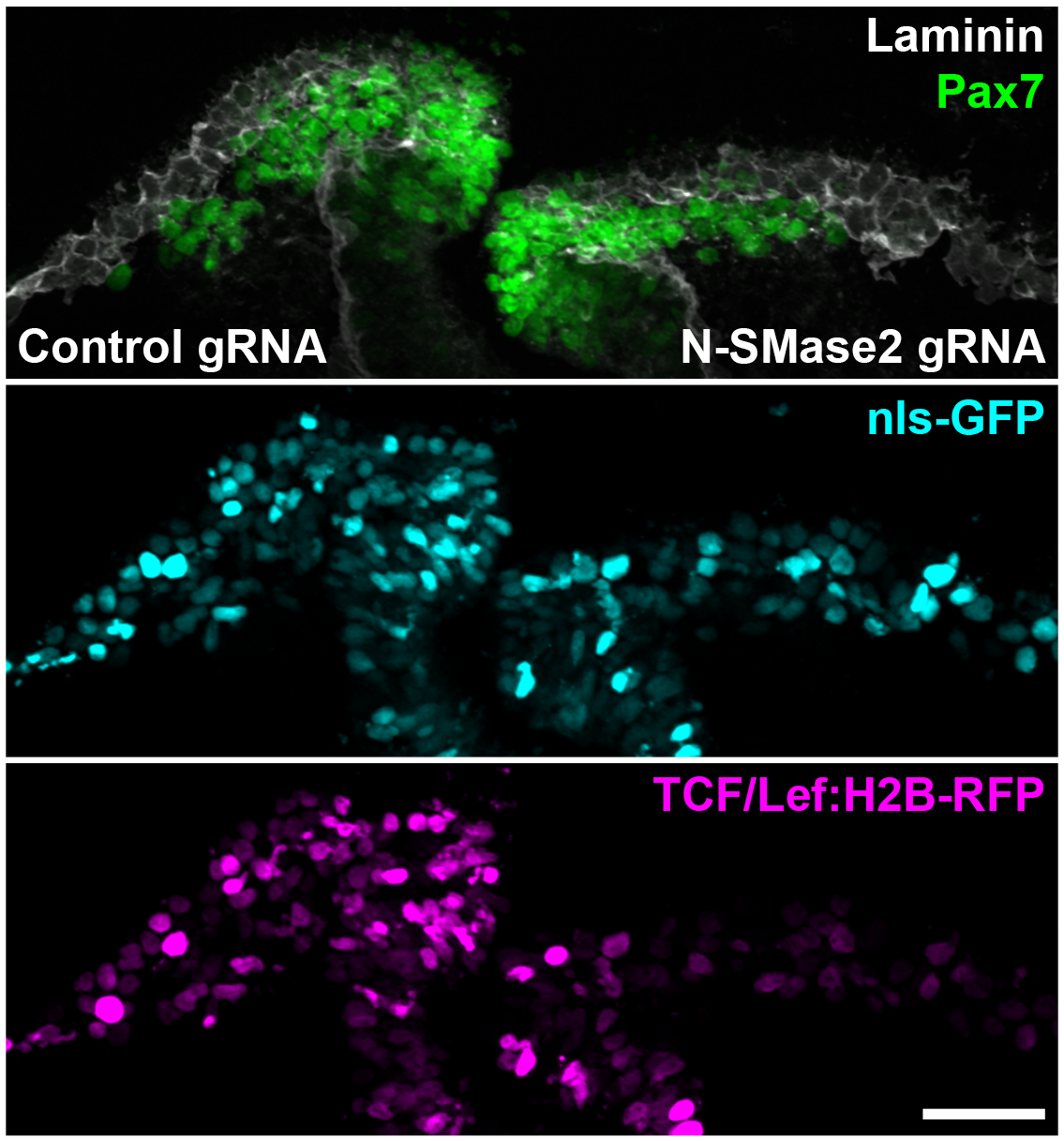
The Bronner lab has found that SMPD3 is enriched in cranial neural crest cells in early development (≈36 hours post-fertilization) of chick embryos (as published here). In current experiments, Mike Piacentino and our very own Cece Andrews in the lab is investigating the role the enzyme nSMase2 (the gene product of SMPD3) may play in Wnt signaling during neural crest cell development in the chick embryo. To address this, Mike performed CRISPR-mediated knockouts of SMPD3 on the right side of developing chick embryos, with a non-binding guide RNA on the left side as a control.
In the experiment, Mike co-electroporated the cells of the cranial neural crest with three molecular species.
Guide RNA: Either a guide RNA allowing for CRISPR knockout of SMPD3 or a control non-binding guide RNA.
pCIG: A vector containing a nuclear localization sequence GFP (nls-GFP), which is used to determine electroporation efficiency.
TCF/Lef::H2B-RFP: A fluorophore whose expression is turned on by Wnt signaling. The fluorescent intensity of this fluorophore is used as a direct readout of Wnt signaling strength.
He then fixed the cells and use antibody staining for Laminin (maker of the basal lamina) and Pax7 (a neural crest marker).
The images below show a typical output of the microscopy experiment. The top image depicts the cells being analyzed. Those showing strong Pax7 signal (green) are cranial neural crest cells and the white Laminin signal shows the basal lamina, essentially serving to provide an outline of the cells. The right side of the image was electroporated with the guide RNA for SMPD3 knockout, and the left side was electroporated with the control non-binding guide RNA. The middle image shows the efficacy of the electroporation; brighter signal means better more effective electroporation. The bottom image shows a readout of Wnt signaling strength, with brighter signal corresponding to stronger Wnt signaling. (Scale bar 100 µm.)
To analyze the images, Mike used ImageJ to hand-draw a closed curve around a given region of interest (ROI). For example, when analyzing the control cells, he drew a closed curve around the collection of cells with strong Pax7 signal on the left half of the image. He also drew ROIs around regions of the image away from the embryo to establish the background fluorescence in the respective channels. He then ran a script based on these drawn ROIs, also with ImageJ, to sum up the relevant pixel values within the ROIs. For each image stack (three images, one from each channel (Pax7, nls-GFP, and TCF/Lef::H2B-RFP)) ImageJ saves a CSV file with the results.
Your job in this problem is to parse multiple CSV files from a collection of images into a single data frame, and then use that data frame to make an instructive graphic of the results. The CSV files can be downloaded here as a ZIP file.
The file naming convention of the CSV files encodes metadata for each experiment, separated by underscores. The convention is best seen by considering one of the files as an example. For the file 20180616_SMPD3crispr_Pax7,Laminin,TCFLefRFP,pCIG_Emb1_9ss_20x_sec1.csv, the respective fields have the following meaning.
20190616: The date of the experimentSMPD3crispr: TreatmentPax7,Laminin,TCFLefRFP,pCIG: The species that represented in the fluorescent channels of the images.Emb1: Embryo number9ss: The somite stage (this is an agreed-upon scale for quantifying the age of the embryo).20x: The magnificationsec1: Section number
Each row of the CSV corresponds to a single region of interest (ROI) of the image. Each CSV file has the following columns.
The index (unnamed in the header row). (Some CSV files explicitly have a column for the index, and this is an example of such a file.)
Label. This is an annotation of which ROI was used for the values in the row.TCFLef:Cntl: TCF/Lef::H2B-RFP channel on the control (left) side of the cranial neural crest.TCFLef:Expt: TCF/Lef::H2B-RFP channel on the knockout (right) side of the cranial neural crest.TCFLef:background: TCF/Lef::H2B-RFP channel with an ROI from a portion of the image that is outside of the embryo.pCIG:Cntl: nls-GFP channel on the control (left) side of the cranial neural crest.pCIG:Expt: nls-GFP channel on the knockout (right) side of the cranial neural crest.pCIG:background: nls-GFP channel with an ROI from a portion of the image that is outside of the embryo.
Area. The area of the ROI in units of square pixels.Mean. The mean intensity for each pixel within the ROI.IntDen. The product of theAreaandMeancolumns.RawIntDen. The sum of the values of all pixels in the ROI prior to image preprocessing (this may be ignored).
a) For each treatment (control or knockout) in each image, do the following.
Compute the mean intensity of the background pixels.
Subtract this mean background intensity from both the control and experiment mean pixel intensity.
Compute the ratio of the background-subtracted mean intensity. That is, compute \((I_\mathrm{TCFLef} - I_\mathrm{TCFLef}^\mathrm{background})/(I_\mathrm{pCIG} - I^\mathrm{background}_\mathrm{pCIG})\), where \(I\) stands for intensity.
Thus, for each image, you get two of these ratios, one for the control (left side) and one for the knockout (right side). (The reason we compute a ratio is because we are scaling the signal by the electroporation efficiency.) Put these processed results in their own data frame.
b) Make an informative plot showing the results you computed in part (a).