Melting a data frame

Data set download

---

import pandas as pd

import bebi103

import bokeh.io
import bokeh_catplot

bokeh.io.output_notebook()

Loading BokehJS ...

You should install the xlrd package to enable Pandas to read in MS Excel file. Before running this lesson, execute the following on the command line.

conda install xlrd

---

In this tutorial, we will perform some wrangling on a data set that involves:

• Using Pandas’s read_excel() function to read in data from an MS Excel spread sheet

• Parsing column names to extract useful metadata en route to tidy data

• Performing a melt operation to efficiently tidy a data set.

The data set

We will use a data set from Angela Stathopoulos’s lab, acquired to study morphogen profiles in developing fruit fly embryos. The original paper is Reeves, Trisnadi, et al., Dorsal-ventral gene expression in the Drosophila embryo reflects the dynamics and precision of the Dorsal nuclear gradient, Dev. Cell., 22, 544-557, 2012, and the data set may be downloaded here.

In this experiment, Reeves, Trisnadi, and coworkers measured expression levels of a fusion of Dorsal, a morphogen transcription factor important in determining the dorsal-ventral axis of the developing organism, and Venus, a yellow fluorescent protein along the dorsal/ventral- (DV) coordinate. They put this construct on the third chromosome, while the wild type dorsal is on the second. Instead of the wild type, they had a homozygous dorsal-null mutant on the second chromosome. The Dorsal-Venus construct rescues wild type behavior, so they could use this construct to study Dorsal gradients.

Dorsal shows higher expression on the ventral side of the organism, thus giving a gradient in expression from dorsal to ventral which can be ascertained by the spatial distribution of Venus fluorescence intensity.

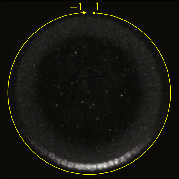
This can be seen in the image below, which is a cross section of a fixed embryo with anti-Dorsal staining. The bottom of the image is the ventral side and the top is the dorsal side of the embryo. The DV coordinate system is defined by the yellow line. The image is adapted from the Reeves, Trisnadi, et al. paper.

A quick note on nomenclature: Dorsal (capital D) is the name of the protein product of the gene dorsal (italicized). The dorsal (adjective) side of the embryo is its back. The ventral side is its belly. Dorsal is expressed more strongly on the ventral side of the developing embryo. This can be confusing.

To quantify the gradient, Reeves, Trisnadi, and coworkers had to first choose a metric for describing it. They chose to fit the measured profile of fluorescence intensity with a Gaussian peak (plus background) and use the standard deviation of that Gaussian as a metric for the width of the Dorsal gradient.

In this lesson, we will use the gradient widths as outputted from this procedure. The units of the widths are dimensionless, consistent with the coordinate system shown in the image above. I asked one of the authors for the data sets used in making the figures. She sent me a MS Excel file that had a separate sheet for each of several figures in the paper that I asked about. We will focus on the data used for Fig. 1F of the paper. In this figure, the authors seek to demonstrate that live imaging with their Venus-Dorsal construct gives a Dorsal gradient of similar width as would be obtained by fixing wild type cells and doing Dorsal antibody staining (the gold standard). These wild type embryos were analyzed as whole mounts and also as cross sections. They also tried anti-Dorsal staining and anti-Venus staining in the Venus-Dorsal construct. Finally, they also measured gradient widths of a GFP-Dorsal construct that fails to complete development.

Loading in an Excel sheet

Generally, you should store your data sets in portable formats, like CSV, JSON, XML, HDF5, ONE-TIFF, etc., and not proprietary formats. Nonetheless, software like Microsoft Excel is widely used, and you will often receive data sets in this format. Fortunately, Pandas can read Excel files, provided they are from fairly recent versions of Excel.

To read in this data set, we will use pd.read_excel(). Importantly, because an Excel document may have many sheets, we need to specify the sheet name we want, in this case 'Fig 1F'.

df = pd.read_excel('../data/Reeves2012_data.xlsx', sheet_name='Fig 1F')

df.head()

	wt wholemounts	wt cross-sections	anti-Dorsal dl1/+dl-venus/+	anti-gfp dl1/+dl-venus/+	Venus (live) dl1/+dl-venus/+	anti-Dorsal dl1/+dl-GFP/+	anti-gfp dl1/+dl-GFP/+	GFP (live) dl1/+dl-GFP/+
0	0.1288	0.1327	0.1482	0.1632	0.1666	0.2248	0.2389	0.2412
1	0.1554	0.1457	0.1503	0.1671	0.1753	0.1891	0.2035	0.1942
2	0.1306	0.1447	0.1577	0.1704	0.1705	0.1705	0.1943	0.2186
3	0.1413	0.1282	0.1711	0.1779	NaN	0.1735	0.2000	0.2104
4	0.1557	0.1487	0.1342	0.1483	NaN	0.2135	0.2560	0.2463

The data frame is not tidy. Each entry corresponds to one observation, not each row. The column headings contain important metadata, the genotype (wt, dl1/+dl-venus/+, or dl1/+dl-GFP/+) and the method (wholemounts, cross-sections, anti-Dorsal, anti-gfp, Venus (live), and GFP (live)).

The data set has other issues we need to clean up. The column 'anti-gfp dl1/+dl-venus/+' is mislabeled; it should be 'anti-Venus dl1/+dl-venus/+'. We would also like to clean up the genotypes, putting in a semicolon to separate the chromosomes. The wild type columns have the genotype first ('wt') followed by the method, whereas the other columns have the method first, followed by genotype.

Parsing the column names

We will start our process of tidying this data set by changing the column names. They are pretty messy, so this is best done by hand in this case. We will rename the columns with tuples to more easily delineate genotypes and methods.

col_names = {
    'wt wholemounts': ('WT', 'whole mount'),
    'wt cross-sections': ('WT', 'cross-section'),
    'anti-Dorsal dl1/+dl-venus/+': ('dl1/+ ; dl-venus/+', 'anti-Dorsal'),
    'anti-gfp dl1/+dl-venus/+': ('dl1/+ ; dl-venus/+', 'anti-Venus'),
    'Venus (live)  dl1/+dl-venus/+': ('dl1/+ ; dl-venus/+', 'Venus (live)'),
    'anti-Dorsal  dl1/+dl-GFP/+': ('dl1/+ ; dl-gfp/+', 'anti-Dorsal'),
    'anti-gfp  dl1/+dl-GFP/+ ': ('dl1/+ ; dl-gfp/+', 'anti-GFP'),
    'GFP (live)  dl1/+dl-GFP/+': ('dl1/+ ; dl-gfp/+', 'GFP (live)')
}

df = df.rename(columns=col_names)

df.head()

	(WT, whole mount)	(WT, cross-section)	(dl1/+ ; dl-venus/+, anti-Dorsal)	(dl1/+ ; dl-venus/+, anti-Venus)	(dl1/+ ; dl-venus/+, Venus (live))	(dl1/+ ; dl-gfp/+, anti-Dorsal)	(dl1/+ ; dl-gfp/+, anti-GFP)	(dl1/+ ; dl-gfp/+, GFP (live))
0	0.1288	0.1327	0.1482	0.1632	0.1666	0.2248	0.2389	0.2412
1	0.1554	0.1457	0.1503	0.1671	0.1753	0.1891	0.2035	0.1942
2	0.1306	0.1447	0.1577	0.1704	0.1705	0.1705	0.1943	0.2186
3	0.1413	0.1282	0.1711	0.1779	NaN	0.1735	0.2000	0.2104
4	0.1557	0.1487	0.1342	0.1483	NaN	0.2135	0.2560	0.2463

Because we named them with tuples, we can reset the column index to be a multiindex using pd.MultiIndex.from_tuples().

df.columns = pd.MultiIndex.from_tuples(df.columns, names=('genotype', 'method'))

df.head()

genotype	WT		dl1/+ ; dl-venus/+			dl1/+ ; dl-gfp/+
method	whole mount	cross-section	anti-Dorsal	anti-Venus	Venus (live)	anti-Dorsal	anti-GFP	GFP (live)
0	0.1288	0.1327	0.1482	0.1632	0.1666	0.2248	0.2389	0.2412
1	0.1554	0.1457	0.1503	0.1671	0.1753	0.1891	0.2035	0.1942
2	0.1306	0.1447	0.1577	0.1704	0.1705	0.1705	0.1943	0.2186
3	0.1413	0.1282	0.1711	0.1779	NaN	0.1735	0.2000	0.2104
4	0.1557	0.1487	0.1342	0.1483	NaN	0.2135	0.2560	0.2463

This is looking better; we have consistent naming of the genotypes and methods and they are organized as a multiindex.

Melting the data frame

When we melt the data frame, the data within it, called values, become a single column. The column names, called variables also become new columns. So, to melt it, we need to specify what we want to call the values and what we want to call the variable. The melt() method does the rest!

df = pd.melt(df, value_name='gradient width')

df.head()

	genotype	method	gradient width
0	WT	whole mount	0.1288
1	WT	whole mount	0.1554
2	WT	whole mount	0.1306
3	WT	whole mount	0.1413
4	WT	whole mount	0.1557

Nice! We now have a tidy data frame.

Note that pd.melt() has other options. For example, you can specify columns that do not comprise data, but should still be included in the melted data frame using the id_vars keyword argument. That does not apply to this data frame, but comes up often.

Deleting NaN’s

The only problem is that it has many NaNs because there were many of them in the data set due to the unequal column lengths in the original spreadsheet. We can see this by looking at the tail of the data frame.

df.tail()

	genotype	method	gradient width
1211	dl1/+ ; dl-gfp/+	GFP (live)	NaN
1212	dl1/+ ; dl-gfp/+	GFP (live)	NaN
1213	dl1/+ ; dl-gfp/+	GFP (live)	NaN
1214	dl1/+ ; dl-gfp/+	GFP (live)	NaN
1215	dl1/+ ; dl-gfp/+	GFP (live)	NaN

We can now safely delete any row that has a NaN.

df = df.dropna()

…and we are good to do with a tidy DataFrame!

Using the data frame

Let’s make a plot like Fig. 1F of the Reeves, Trisnadi, et al. paper, but not with boxes, rather as a strip plot. We will use Bokeh-catplot because HoloViews does not yet allow for nested categorical axes with a scatter plot.

p = bokeh_catplot.strip(
    data=df,
    cats=['genotype', 'method'],
    val='gradient width',
    color_column='genotype',
    horizontal=True,
    jitter=True,
    frame_height=350,
    frame_width=450,
)

bokeh.io.show(p)

Computing environment

%load_ext watermark
%watermark -v -p pandas,bokeh,bokeh_catplot,jupyterlab

CPython 3.7.4
IPython 7.8.0

pandas 0.24.2
bokeh 1.3.4
bokeh_catplot 0.1.6
jupyterlab 1.1.4