R6. Probability review¶

This document was prepared by Ankita Roychoudhury with help and suggestions from Rosita Fu.

[1]:

# Colab setup ------------------
import os, sys, subprocess
if "google.colab" in sys.modules:
    cmd = "pip install --upgrade watermark"
    process = subprocess.Popen(cmd.split(), stdout=subprocess.PIPE, stderr=subprocess.PIPE)
    stdout, stderr = process.communicate()
    data_path = "https://s3.amazonaws.com/bebi103.caltech.edu/data/"
else:
    data_path = "../data/"
# ------------------------------

import pandas as pd

import numpy as np

import iqplot
import bebi103

rg = np.random.default_rng()

import bokeh.io
import bokeh.plotting.figure
import bokeh.layouts
bokeh.io.output_notebook()

import holoviews as hv
hv.extension('bokeh')
bebi103.hv.set_defaults()

Loading BokehJS ...

In this recitation, we will cover:

Review of Important Probability Concepts

Frequentist interpretation
Marginalization
Plug-in estimates of parameters
Confidence intervals
Parametric vs nonparametric inference

Probability Distributions (Properties)

Examples
PMF vs PDF vs CDF vs ECDF
Random number generation

Other

Kolmogorov’s 0-1 law

Review¶

We will begin by reviewing some basic concepts in probability.

Frequentist interpretation¶

Given a sample (such as time of sleeping fish, fluorescence values, lengths of C. elegans eggs), you can extract summary metrics to describe it (such as average, variance, etc). These quantities help us understand the summarize only the sample.

What if I want to understand how all C. elegans egg lengths vary with different treatments, i.e. something more general than what is displayed in the sample? This is called inferential statistics.

Why use inferential statistics?

parameter estimation
data prediction
model comparison

Frequentist - Probably can only be ascribed to random variables, which are quantities that can very meaningfully from experiment to experiment. The probability of an event is the long-term frequency of that event.

Bayesian - Can use probabilities to describe uncertainty to any event, even non-repeatable ones. Can apply prior knowledge. You have more freedom when using a Bayesian mindset!

Marginalization¶

Marginalization is the process of summing over the possible values of one variable (often one that is difficult to measure) to determine its marginal contribution to the other. Each element has different weights.

Let’s consider an example where you grew some plants in your backyard and are trying to understand the probability of them surviving.

Weather	Plant Condition	Probability
sunny	dead	x
sunny	alive	y
cloudy	dead	z
cloudy	alive	a
rainy	dead	b
rainy	alive	c

Now, let’s assume we want to marginalize out the dependence on weather. Then, our table would read something like this:

Plant Condition	Probability
dead	d
alive	e

See how much simpler that is? We can encode information about the weather into the resulting growth condition. Note that \(x + y + z + a + b + c = 1\) and \(d + e = 1\). To find \(d\) and \(e\), we can sum the corresponding probabilities they are made up of. For example, \(P(\text{dead}) = P(\text{sunny}, \text{dead}) + P(\text{cloudy}, \text{dead}) + P(\text{rainy}, \text{dead}) = x + z + b\). We are summing (or integrating in the continuous case) over a particular variable—we are calculating the marginal contribution of that variable in order to “get rid” of it (aka we no longer need to explicitly account for it).

Parametric parameter estimates¶

Given a data set, let’s say we pick a distribution by which we think the data is modeled. For the Normal distribution, we may want to have estimations for the mean and the variance, the parameters by which that distribution is governed. Let’s take the finch data set for example.

[2]:

# Load file and take a look
df = pd.read_csv(os.path.join(data_path, "finch_beaks.csv"))
df.head()

[2]:

	band	beak depth (mm)	beak length (mm)	species	year
0	20123	8.05	9.25	fortis	1973
1	20126	10.45	11.35	fortis	1973
2	20128	9.55	10.15	fortis	1973
3	20129	8.75	9.95	fortis	1973
4	20133	10.15	11.55	fortis	1973

Let’s consider the finch beak depths for all yaers.

[3]:

p = iqplot.histogram(data=df, q="beak depth (mm)", title="Finch Beak Depths")
bokeh.io.show(p)

This histogram shows our empirical distribution, a distribution associated with a collection of samples.

To fully specify a Normal distribution, we need a location and scale parameter (see Probability Distribution Explorer). Given our data set, we can compute estimates for these as the sample mean and variance. As we will derive later in the course, the plug-in estimates for the Normal distribution happen to be good ones (they are specifically maximum likelihood estimates, which we will define in coming lessons).

[4]:

depth_vals = df["beak depth (mm)"].values

mean = np.average(depth_vals)
variance = np.var(depth_vals)

print("The mean is:", mean, "mm")
print("The variance is:", variance, "mm²")

The mean is: 9.208625489343191 mm
The variance is: 0.5641561794459872 mm²

With this information, we can take a look at what the data set would look like if it were generated from a Normal distribution with these parameters.

[5]:

generated_data = rg.normal(mean, np.sqrt(variance), size=len(depth_vals))

p1 = iqplot.histogram(
    data=generated_data,
    title="Theoretical Finch Beath Depths",
    fill_kwargs={"fill_color": "#e34a33"},
    line_kwargs={"line_color": "#e34a33"},
)
bokeh.io.show(p1)

Let’s overlay the two plots (and overlay the two ECDFs).

[6]:

# Get combined histogram
p2 = iqplot.histogram(
    data=generated_data,
    p=p,
    fill_kwargs={"fill_color": "#feb24c"},
    line_kwargs={"line_color": "#feb24c"},
)
p2.title.text = "Overlay of Generated and Sample Finch Beak Depth Histograms"

# Get ECDF of actual data
p3 = iqplot.ecdf(data=df, q="beak depth (mm)", title="Finch Beak Depths")

# Get combined ECDF
p4 = iqplot.ecdf(
    data=generated_data,
    p=p3,
    marker_kwargs={"line_color": "#feb24c", "fill_color": "#feb24c"},
)
p4.title.text = "Overlay of Generated and Sample Finch Beak Depth ECDFs"

# Take a look
bokeh.io.show(bokeh.layouts.row(p2, p4))

Are the data from the putative generative model close to those that were actually measured? Sure looks like it. This is a question we will delve into later this term… and a lot more next term!

Confidence Intervals¶

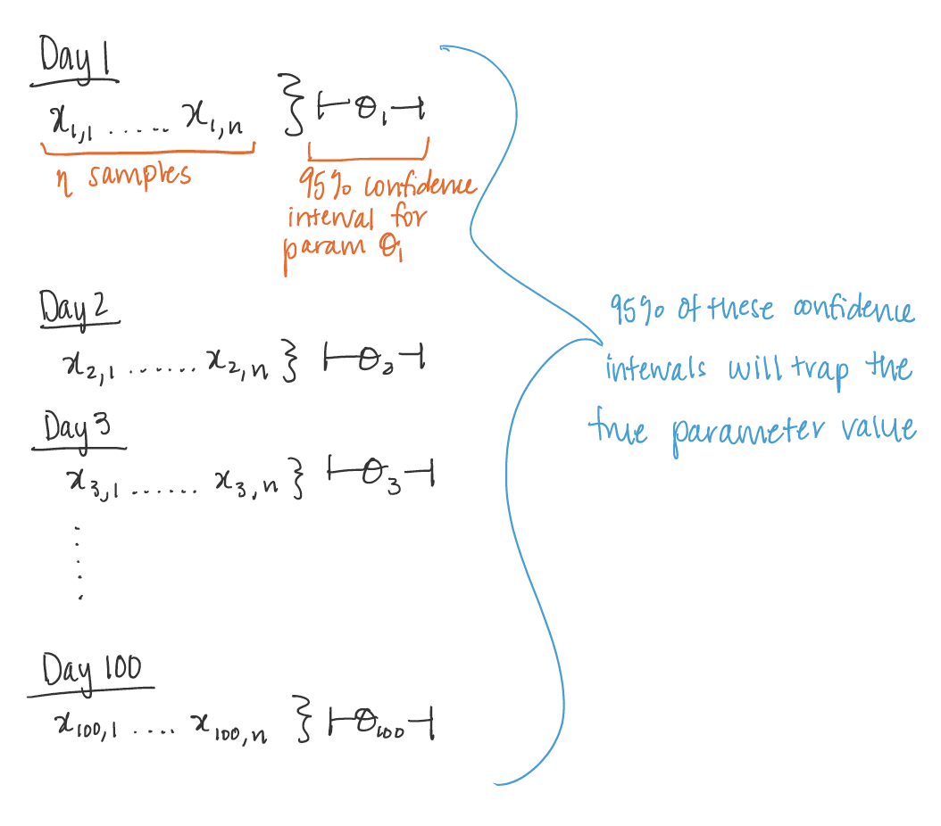
A confidence interval is not just “a range of values we are fairly sure our true value lies in.” Which is unfortunately the first result when I Google search “what is a confidence interval.” They use the mean height of 40 men as their example.

Let’s clarify! As Larry Wasserman writes (see Lesson 12),

On day 1, you collect data and construct a 95 percent confidence interval for a parameter 𝜃1. On day 2, you collect new data and construct a 95 percent confidence interval for an unrelated parameter 𝜃2. On day 3, you collect new data and construct a 95 percent confidence interval for an unrelated parameter 𝜃3. You continue this way constructing confidence intervals for a sequence of unrelated parameters 𝜃1, 𝜃2,…. Then 95 percent of your intervals will trap the true parameter value.

Nice! Let’s visualize it.

Parametric vs Nonparametric Inference¶

Parametric Inference - Explicitly models the generative distribution.

Nonparametric Inference - Does not explicitly model the generative distribution.

Probability Distributions¶

Examples¶

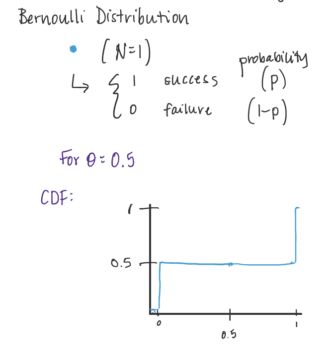
Bernoulli Distribution¶

A Bernoulli Distribution describes the result of a single Bernoulli trial. It can either be a success or a fail.

Parameter: \(\theta\) = probability of the trial being successful.

Visualize:

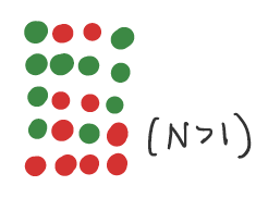
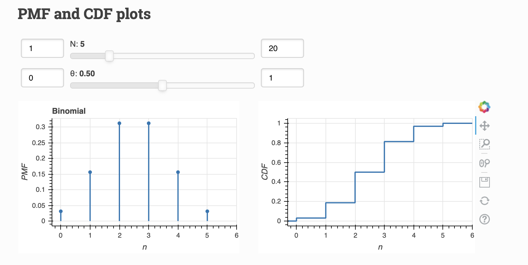
Binomial Distribution¶

A Binomial Distribution describes the result of \(N\) Bernoulli trials. The number of successes \(n\), is Binomially distributed.

Parameters:
- \(\theta\) = probability of the trial being successful
- \(N\) = number of total trials

Visualize:

Geometric Distribution¶

Perform a series of Bernoulli trials with probability of success \(\theta\) until a success. The number of failures \(y\) before the success is Geometrically distributed. * Parameter: \(\theta\) = probability of one trial being successful.

Visualize:

Poisson Distribution¶

The number of arrivals, \(n\), of a Poisson process in unit time is Poisson distributed. - Parameter: \(\lambda\) = rate of arrival of the Poisson Process

PMF vs PDF vs CDF vs ECDF¶

It’s easy to get confused by these acronyms so let’s lay it out explicitly just in case, because the differences are important!

First, see if the distribution you are working with is for discrete or continuous variables.

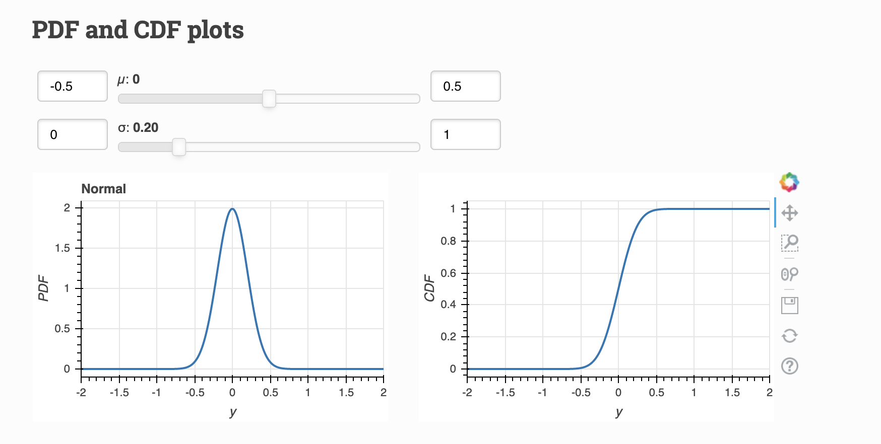
Continuous (PDF, CDF)¶

A continuous random variable has a infinite, uncountable range in which values can fall (ex. length of C. elegans eggs).

The PDF represents the probability density of a continuous variable. The CDF is the derivative of the PDF.

Visualize:

Discrete (PMF, CDF)¶

A discrete random variable takes on certain values (ex. coin flips can be either 0 or 1).

The PMF represents the probability that a value is equal to a discrete value.

The CDF is the derivative of the PMF.

Visualize:

Both visualizations from Distribution Explorer.

CDF vs ECDF¶

A CDF always corresponds to a hypothetical model of a distribution.

The ECDF always comes from empirical or observed data.

Random Number Generation is powerful!¶

There are so many things we can do with rng… like random walks! (which are seen everywhere in biology)

Let’s do a 2D random walk with 10000 steps (code from lesson 10).

[7]:

# Get parameters and x,y values
n_steps = 10000
theta = rg.uniform(low=0, high=2*np.pi, size=n_steps)

x = np.cos(theta).cumsum()
y = np.sin(theta).cumsum()

Plot!

[8]:

hv.extension("bokeh")

hv.operation.datashader.datashade(
    hv.Path(
        data=(x, y),
        kdims=['x', 'y']
    )
).opts(
    frame_height=300,
    frame_width=300,
    padding=0.05,
    show_grid=True,
    title = 'Random Walk with RNG'
)

[8]:

How cool! Imagine all the processes we can model with this tool!

Misc. Topics¶

Kolmogorov’s 0-1 Law¶

A tail event occurs with probability 0 or 1.