R2. Review of MLE
This recitation was prepared by Rosita Fu.
Although we will not be doing anymore MLE this term, the analytical and numerical techniques we learned last term will translate well to some of our objectives this term. We will review what the MLE is, how to find it analytically and numerically, and see how this helps us construct confidence intervals for our parameters.
Review of BE/Bi 103 a lessons
The relevant BE/Bi103a lessons are linked, but they are essentially lessons 19, 20, and 22.
MLE Introduction: notes
Numerical MLE: notes
MLE Confidence Intervals: notes
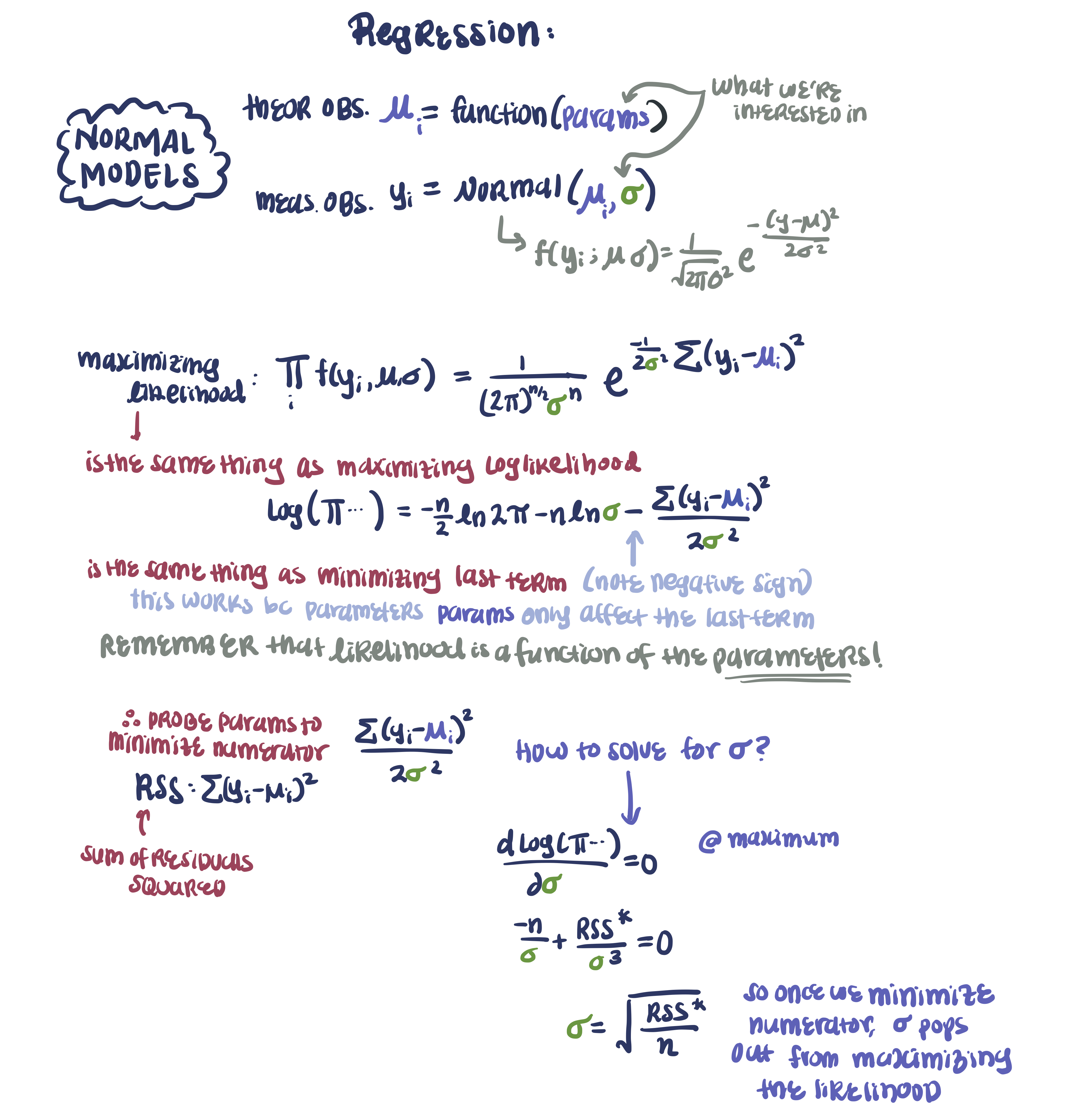
Regression: normal MLE & regression
For those who are just joining us this term, if time allows, to understand confidence intervals, it might be helpful to review what bootstrapping is. If the distributions themselves are new to you, you will become intimately familiar with them by the end of this term, so I wouldn’t worry too much. I would recommend bookmarking distribution-explorer.github.io, or visiting the link so many times all you have to do is type ‘d’ + ‘enter’.
def log_likelihood(...) function that works.scipy.optimize.minimize(...) function with kywargs:fun: lambda parameters x0: initial guess for parameters of type array, (order should match the log_likelihood function you defined)method: either ‘BFGS’ or ‘Powell’ 3. Add warning-filters and retrieve parametersNotes
Following are notes to accompany recitation. If you are already familiar with MLE, I suggest jumping to the last section (parameter estimation).
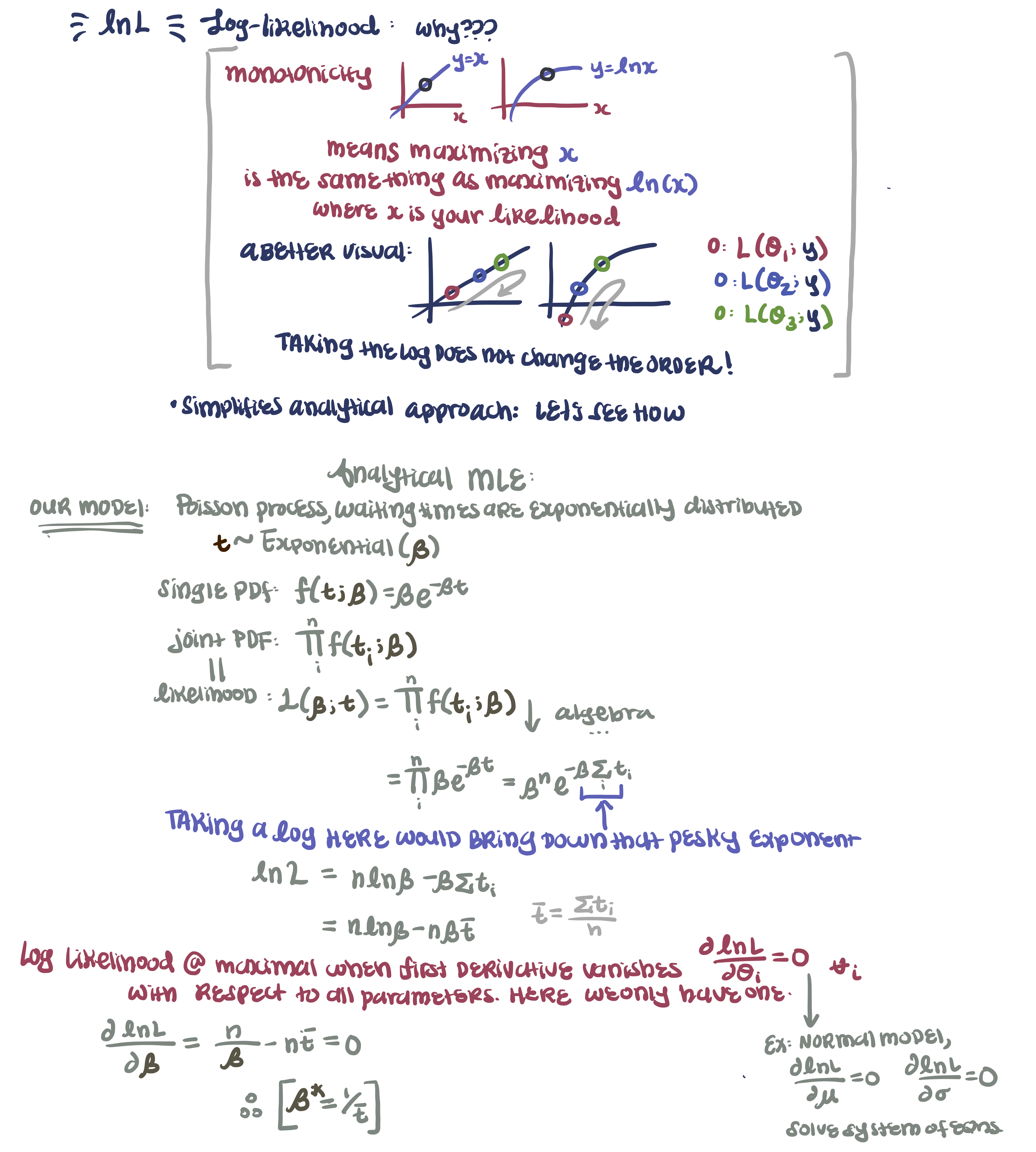
Numerical MLE for mortals tend to be somewhat challenging, so we are always on the look-out for more elegant approaches (or at the very least, doing as much work analytically as we can to make the computation a smoother process). For a likelihood constructed from a normal distribution, we can apply a very nice property that maximizing the likelihood is functionally equivalent to minimizing the residuals. I include my notes here as a reminder of the sensibility of least squares with a particular distribution: the Normal.
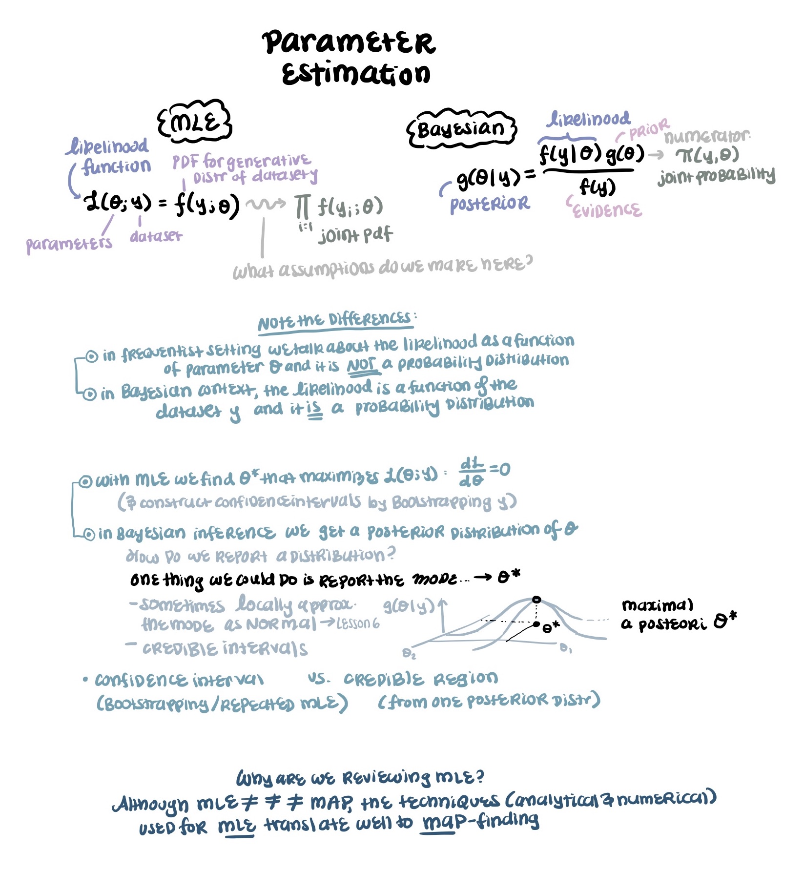
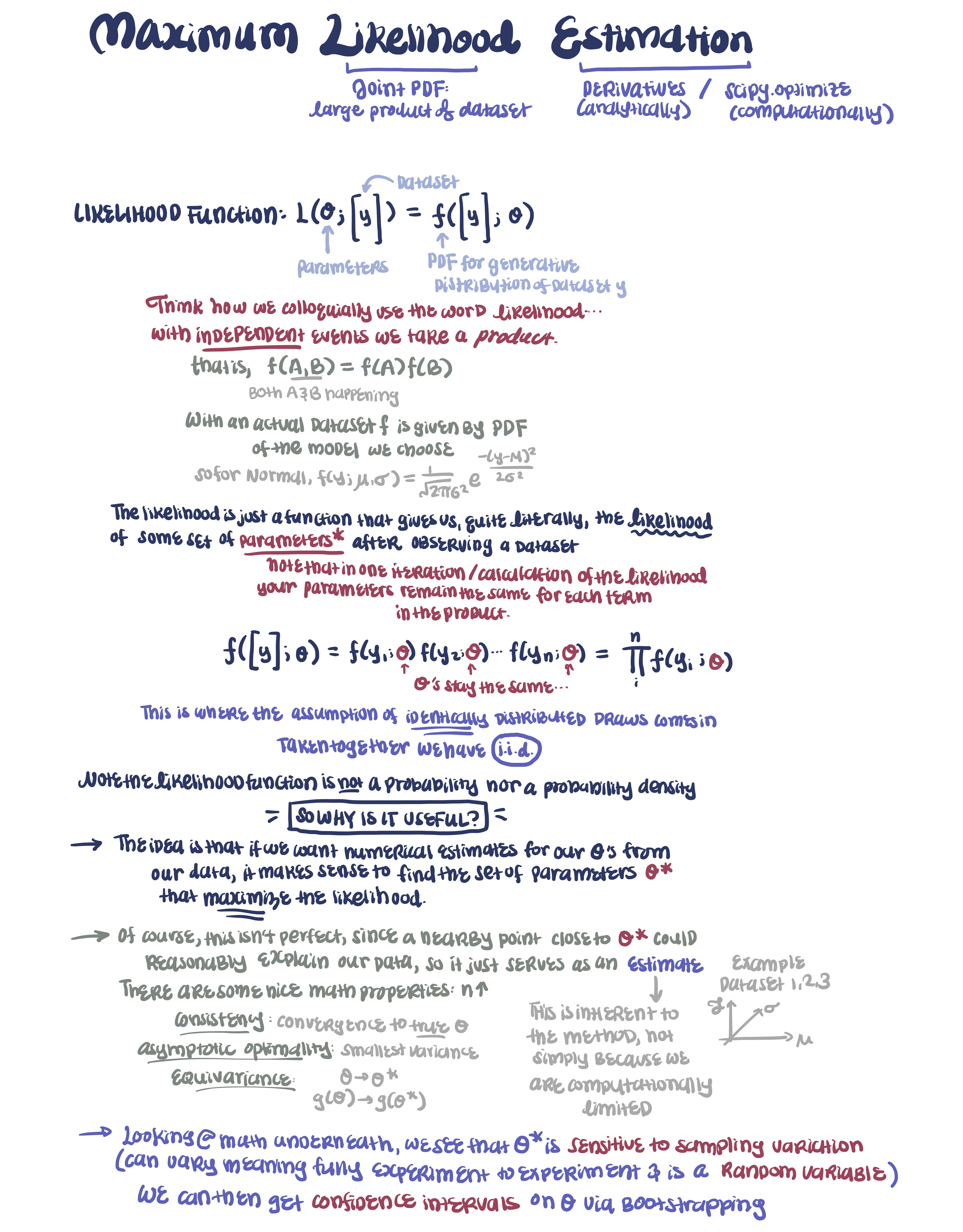
At its very core, the MLE likelihood is a function of its parameters, and its maximization is motivated by the following: “among all explanations from the observed data, choose as best the one that makes the data most probable.”
As you have learned this past week, the likelihood in Bayesian modeling is defined differently: it is merely the (conditional) probability of observing our dataset conditioned on a set of parameters, and sits in the numerator. Bayes’ law proceeds to give us a posterior distribution for our parameter, and summarizing this posterior with a MAP and/or credible interval is analagous to reporting an MLE with a confidence interval.
I hope you can see that the Bayesian likelihood encodes how our data is generated, but it is an intermediate figure in our parameter estimation—what is of interest in the end is our posterior, whereas the MLE likelihood is directly the thing we maximize.
One last note: although numerically, the MLE/Bayesian likelihood may give us the same value for a given \(\theta\), they mean different things, and come from different places. Recall above where we took a joint pdf in the MLE, and made the i.i.d. assumption to justify taking a product (can only do this for independent events). We do not actually need the assumption of independence in a Bayesian context: Bayes’ law is always true! Thus, the data acquisition process can be thought of as presented in Lesson 1. We may, however, still need the identically distributed assumption (though the Bayesian framework offers us a way to explicitly encode parameters we know to be non-identical: this is the essence of hierarchical modeling, and will be introduced towards the end of the course).
I encourage you to read the lessons for a much more thorough introduction and demonstration, but I hope the motivation is somewhat clear, or at the very least, less obscure.