More details on Hamiltonian Monte Carlo

This portion of the recitation was prepared by Tom Röschinger.

---

import numpy as np
from scipy.special import binom, factorial
import scipy.stats as st

import bokeh.plotting
from bokeh.io import curdoc, show
import bokeh.palettes
from bokeh.layouts import row,layout
from bokeh.models.tickers import FixedTicker

import holoviews as hv
renderer = hv.renderer('bokeh')
hv.extension('bokeh')

pallete1 = ['#9faeb2', '#ab6e7d', '#1c2630']

bokeh.io.output_notebook()

BokehJS 3.3.0 successfully loaded.

def style(p, autohide=False):
    p.title.text_font="Helvetica"
    p.title.text_font_size="16px"
    p.title.align="center"
    p.xaxis.axis_label_text_font="Helvetica"
    p.yaxis.axis_label_text_font="Helvetica"

    p.xaxis.axis_label_text_font_size="13px"
    p.yaxis.axis_label_text_font_size="13px"
    p.xaxis.axis_label_text_font_style = "normal"
    p.yaxis.axis_label_text_font_style = "normal"
    p.background_fill_alpha = 0
    if autohide: p.toolbar.autohide=True
    return p

---

This recitation will be heavily based on this paper by Michael Betancourt. For anyone interested in the background of this complex topic, I recommend reading the paper. I will do my best to break it down here. We will start of by introducing some of the key components, such as typical sets and the physical meaning of a Hamiltonian.

The typical set

The typical set is a subset of the sample space that contains most of the probability mass. In general, this set does not contain the most likely outcome. For a more detailed explanation, check out Bob Carpenter’s explanation. Let’s look at the Binomial distribution as an example. We perform $N=500$ successive Bernoulli trials for a variable $y\in \{0,1\}$ with probability $\theta =0.75$ to get $y=1$. The most probable sequence of outcomes is $\mathbf{y}=(1,1,...,1)$. If we are only interested in the number of successes however, this outcome is very unlikely. This is because we have to weigh the number of successes with the number of possible outcomes that give that result. That’s why the binomial coefficient is included in the Binomial distribution. It is much more likely to draw a number of successes that is close to the expectation value, $⟨y⟩=N\theta =375$. To get a feeling of how the outcomes would be distributed, imagine you draw a million times from this Binomial. On average, only one (!) draw will be outside the region [326, 420].

N = 500
θ = 0.75

x = np.arange(0, N)

# Compute binomial coefficient
binomial_coeff = binom(N, x)
prob = [θ**n * (1-θ)**(N-n) for n in x]
P = prob * binomial_coeff

# Rescale for plotting
binomial_coeff = binomial_coeff / np.max(binomial_coeff)
prob = prob / np.max(prob)
P = P / np.max(P)

# Make plot
p = bokeh.plotting.figure(frame_width=450, frame_height=300, x_axis_label="n",
    title="N={}, θ={}".format(N, θ), y_range=(-0.05, 1.05))
p.patch([326, 326, 420, 420],[-0.2, 1.2, 1.2, -0.2], color="#eaeaea")
p.line(x, binomial_coeff, line_width=2.2, color=pallete1[0], legend_label="Degeneracy")
p.line(x, prob, line_width=2.2, color=pallete1[1], legend_label="p^n (1-p)^(N-n)")
p.line(x, P, line_width=2.2, color=pallete1[2], legend_label="Typical Set")
p.legend.location = "top_left"

bokeh.io.show(style(p))

a = st.binom.ppf(5*10**-7, N, θ)
b = st.binom.ppf(1-5*10**-7, N, θ)
print("999999 out of 1000000 draws are between {} and {} (on average).".format(a, b))

999999 out of 1000000 draws are between 326.0 and 420.0 (on average).

So why is this important? All of the computations of interest in Bayesian statistics are formulated as expectations over the posterior, for example.

$$⟨\theta ⟩=\int \mathrm{d}\theta \theta p(\theta |y).$$

Technically, we need to compute this integral over the entire sample space. However, since most probability mass is concentrated in the typical set, this integral is very well approximated by an integral, where we only evaluate the posterior density in the typical set (which I labeled $\mathcal{A}$ below),

$$⟨\theta ⟩\approx {\int }_{\theta \in \mathcal{A}}\mathrm{d}\theta \theta p(\theta |y).$$

The higher the dimension, the more crucial it is to find the typical set to compute expectations. This is due to the fact that most of the sample space density is away from the typical set, and this imbalance increases heavily with the dimensionality.

In practice we compute expectations by sampling. Instead of computing the integral numerically, we draw (effectively) independent samples from the distribution. This is especially useful in the cases where we don’t know the exact form of the distribution (which is nearly every case in applications). I won’t review the basics of MCMC here, since this was discussed in class. Now the importance of the typical set becomes even more evident. Instead of needing samples from the entire sample space, which is incredibly huge, we only need to draw samples from the typical set. So our task will be to first find and then sample from the typical set.

Hamiltonians

If you had a Physics course on classical mechanics (or quantum mechanics), this section should be very familiar, but it still works as a refresher. In classical mechanics, the Hamiltonian is the function which describes the total energy of a system. Due to the conservation of energy, this function usually contains all the information of the system, hence it is incredibly powerful. Here we will take a look at the most basic example, the harmonic oscillator. You can imagine this system to be a point mass (it has no volume) with mass $m$ attached to a spring. The strength of the spring is described by a parameter $k$. The force acting on the mass by the spring when it is away from its resting position by a distance $x$ is just $F=-kx$ (negative sign since it points back to the resting position), meaning it is increasing linearly with the distance to the resting position. Force is connected to a potential energy $U$ by a negative derivative, $F=-\partial U/\partial x$, hence we can write down the potential energy $U=k{x}^2/2$.

Since the Hamiltonian is the sum of the total energy, it also contains the kinetic energy of our point mass, which is the contribution to energy from its movement. Kinetic energy is usually written as $T=m{v}^2/2$, where $v$ is the speed of the object. Now we can write down our Hamiltonian:

$$\begin{array}{r}H=T+U=\frac{1}{2}m{v}^2+\frac{1}{2}k{x}^2=\frac{1}{2m}{p}^2+\frac{1}{2}k{x}^2,\end{array}$$

where in the last step we replaced the speed of the object by its momentum, $p=mv$. We will see in a moment why this is a more convenient way of writing the Hamiltonian. Also, I think it is a little more intuitive to think about momentum (Imagine a Fiat 500 hitting a brick wall: the Fiat will probably be a total wreck, since it does not have so much mass. Now imagine a train hitting the same wall with the same speed: the wall will probably not stand a chance, since the train has much more mass. Long story short, think momentum not speed.) The variables $x$ and $p$ define the so called phase space, which is a very important concept in physics.

One of the most important axioms of physics is the conservation of energy. In a closed system, there cannot be any energy generated or consumed, only transformed, therefore $\partial H/\partial t=0$. As a result, for a fixed energy, there is only one free parameter in the equation. That means, that if we choose an energy, then we can choose a value for one of the phase space variables, let’s say the location, and the other variable, in this case momentum, is fixed. (In this case, the resulting plot looks like an ellipsoid).

def simple_oscillator(H, x):
    return np.sqrt(H - x ** 2)

p = bokeh.plotting.figure(
    x_axis_label="x", y_axis_label="p", title="Energy level sets", frame_width=300, frame_height=300,
)
for H, color in zip([9, 4, 1], bokeh.palettes.BuPu[4]):
    x_arr = np.linspace(-np.sqrt(H), np.sqrt(H), 1000)
    p_plus = simple_oscillator(H, x_arr)
    p_minus = -simple_oscillator(H, x_arr)
    p.line(x_arr, p_plus, line_width=2, color=color)
    p.line(x_arr, p_minus, line_width=2, color=color)

legend = bokeh.models.Legend(items=[(f"{H}", [p.line(line_width=2, color=color)])
    for H, color in zip([9, 4, 1], bokeh.palettes.BuPu[4])])
p.add_layout(legend, 'right')
p.legend.title = "H"
p.xaxis.major_label_text_font_size = "0pt"
p.yaxis.major_label_text_font_size = "0pt"

bokeh.io.show(style(p))

This means, that for depending on the energy of the system, the phase space variables will always be on fixed line. These lines are also called trajectories in phase space. Although we do know now how position depends on momentum and vice versa, we still don’t know the time evolution of these variables look like. To do so, we use the absolute beauty of Hamilton’s equations of motion:

$$\begin{array}{r}\frac{\partial p}{\partial t}=-\frac{\partial H}{\partial x},\frac{\partial x}{\partial t}=\frac{\partial H}{\partial p}.\end{array}$$

Applying this to the Hamiltonian of the harmonic oscillator, we obtain

$$\begin{array}{r}\frac{\partial p}{\partial t}=-\frac{\partial H}{\partial x}=-kx,\frac{\partial x}{\partial t}=\frac{\partial H}{\partial p}=p/m.\end{array}$$

We can also compute the equations by using the conservation of energy (which is not something different but rather doing the same thing from a different perspective). Then, by solving for the position we get

$$\begin{array}{r}x=-\frac{1}{k}\frac{\partial p}{\partial t}=-\frac{m}{k}\frac{{\partial }^{2}x}{\partial t^2},\end{array}$$

which is consistent with what we got from using Hamilton’s equations. Now that we have the derivatives in hand, we can compute the trajectories in time,

$$\begin{array}{r}x(t)=x(t_0)+{\int }_{t_0}^t\frac{\partial H}{\partial p}p(t)=p(t_0)-{\int }_{t_0}^t\frac{\partial H}{\partial x}.\end{array}$$

In this case, trajectories in phase space will always look like the ones in the figure above. Any other trajectory requires a change in energy of the system (technically there could be nearly any trajectory, but that would require continuous change in energy). To make this more clear, we can include a vector field into the phase space, which will indicate how allowed trajectories will look like.

xs, ys = np.linspace(-4, 4, 16), np.linspace(-4, 4, 16)
X, Y = np.meshgrid(xs, ys)

# Convert U, V to magnitude and angle
mag = np.sqrt(X**2 + Y**2)
angle = (np.pi/2.0) - np.arctan2(Y / mag, -X / mag)

vectorfield = hv.VectorField(
    (xs, ys, angle, mag)
).opts(
    magnitude='Magnitude',
    height=400,
    width=400,
    #cmap='viridis',
    color='gray',
    xlabel="q",
    ylabel="p",
    alpha=0.6
)

vectorfield

So where ever we start in phase space, the vector fields tells us where to go. And the time evolution is given by Hamilton’s equations.

For illustration purpose, you can download a Bokeh app with small animation of a spring and the resulting trajectory in phase space here. To view the Bokeh app, you can serve it up from the command line by doing

bokeh serve --show oscillator.py

Alternatively, you can enter the above command preceded by a ! in a cell in a Jupyter notebook. You’ll have interrupt the kernel when you are done with the animation.

Hamiltonian Monte Carlo

Let’s put our knowledge of Hamiltonians to use. First we need to choose our Hamiltonian Function, for which we take the log of a joint distribution of both variables,

$$\begin{array}{r}H(q,p)=-\log \pi (q,p)=-\log \pi (p|q)-\log \pi (q).\end{array}$$

In therms of potential and kinetic energy this reads as,

$$\begin{array}{r}H(q,p)=T(q,p)+U(q).\end{array}$$

The trick is to identify $q$ as the parameters of interest and $U(q)=-\log \pi (q)$ as the negative log posterior. Let’s look again and Hamilton’s equations,

$$\begin{array}{r}\frac{\partial q}{\partial t}=\frac{\partial T}{\partial p}\frac{\partial p}{\partial t}=-\frac{\partial T}{\partial q}-\frac{\partial U}{\partial q}\end{array}$$

The only thing we are left with is to choose a kinetic energy. How we choose a kinetic energy will be discussed in the next section. Assume for now that we have chosen a kinetic energy and know its derivative. Then we can compute the trajectories for both momentum and location (our parameters)! As we said before, we want to sample out of the typical set, which means that we want to find a trajectory which follows the typical set. By sampling out of the typical set of the joint distribution we automatically sample out of the typical set of the posterior distribution.

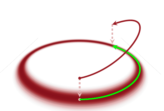
(Image taken from Betancourt, Michael. “A conceptual introduction to Hamiltonian Monte Carlo.” arXiv preprint arXiv:1701.02434 (2017).)

Transition using HMC

Assume we are at a given position in parameter space $q$ (we have an initial condition of parameters), then we need to come up with a kinetic energy function and a set of momenta $p$ (a set because we need one momentum per dimension). Once we made that choice, we can simply use Hamilton’s equations to integrate forward and find a new sample of parameters. As we discussed earlier, that just means that we follow the path in phase space that corresponds to that certain value of energy that we chose. A transition would look something like this.

H = 9
color = bokeh.palettes.BuPu[4][0]
x_arr = np.linspace(-np.sqrt(H), np.sqrt(H), 1000)
p_plus = simple_oscillator(H, x_arr)
p_minus = -simple_oscillator(H, x_arr)

scatter1 = hv.Scatter(([x_arr[100], x_arr[300]], [p_plus[100], p_plus[300]])).opts(
    size=10, color="orange", alpha=0.5
)
scatter2 = hv.Scatter(([x_arr[100], x_arr[300]], [0, 0])).opts(size=10, color="orange")
arrow1 = hv.Curve(([x_arr[100], x_arr[100]], [0, p_plus[100] - 0.1])).opts(
    color="orange", alpha=0.5
)
arrow1_1 = hv.Curve(
    ([x_arr[100] - 0.2, x_arr[100]], [p_plus[100] - 0.3, p_plus[100] - 0.1])
).opts(color="orange", alpha=0.5)
arrow1_2 = hv.Curve(
    ([x_arr[100] + 0.2, x_arr[100]], [p_plus[100] - 0.3, p_plus[100] - 0.1])
).opts(color="orange", alpha=0.5)
arrow2 = hv.Curve(([x_arr[300], x_arr[300]], [0.1, p_plus[300]])).opts(
    color="orange", alpha=0.5
)
arrow2_1 = hv.Curve(([x_arr[300] - 0.2, x_arr[300]], [0.3, 0.1])).opts(
    color="orange", alpha=0.5
)
arrow2_2 = hv.Curve(([x_arr[300] + 0.2, x_arr[300]], [0.3, 0.1])).opts(
    color="orange", alpha=0.5
)
partial_H = hv.Curve((x_arr[100:300], p_plus[100:300])).opts(color="orange", alpha=0.5)
joint = (
    scatter1
    * scatter2
    * vectorfield
    * arrow1
    * arrow2
    * partial_H
    * arrow1_1
    * arrow1_2
    * arrow2_1
    * arrow2_2
)


joint.opts(
    height=400,
    width=400,
    xlim=(-4, 4),
    ylim=(-4, 4),
    show_grid=True,
    xlabel="q",
    ylabel="p",
)

Now we need to use this multiple times to get multiple samples. At each step we need to sample new momenta, and therefore are following a different trajectory in each step. Therefore, we can distinguish HMC sampling into two distinct phases. First, choosing appropriate momenta and kinetic energies, and them numeric integration of the trajectory. At the end of the trajectory we receive a new sample. Let’s take a look at both if these phases and how to do them.

H1 = 9
H2 = 2
H3 = 4

x_arr1 = np.linspace(-np.sqrt(H1), np.sqrt(H1), 1000)
x_arr2 = np.linspace(-np.sqrt(H2), np.sqrt(H2), 1000)
x_arr3 = np.linspace(-np.sqrt(H3), np.sqrt(H3), 1000)

p_plus1 = simple_oscillator(H1, x_arr1)
p_minus1 = -simple_oscillator(H1, x_arr1)
p_plus2 = simple_oscillator(H2, x_arr2)
p_minus2 = -simple_oscillator(H2, x_arr2)
p_plus3 = simple_oscillator(H3, x_arr3)
p_minus3 = -simple_oscillator(H3, x_arr3)

scatter1 = hv.Scatter(([x_arr1[100], x_arr1[300]], [p_plus1[100], p_plus1[300]])).opts(
    size=10, color="orange", alpha=0.5
)
scatter2 = hv.Scatter(([x_arr1[100], x_arr1[300]], [0, 0])).opts(
    size=10, color="orange"
)
arrow1 = hv.Curve(([x_arr1[100], x_arr1[100]], [0, p_plus1[100] - 0.1])).opts(
    color="orange", alpha=0.5
)
arrow1_1 = hv.Curve(
    ([x_arr1[100] - 0.1, x_arr1[100]], [p_plus1[100] - 0.2, p_plus1[100] - 0.1])
).opts(color="orange", alpha=0.5)
arrow1_2 = hv.Curve(
    ([x_arr1[100] + 0.1, x_arr1[100]], [p_plus1[100] - 0.2, p_plus1[100] - 0.1])
).opts(color="orange", alpha=0.5)
arrow2 = hv.Curve(([x_arr1[300], x_arr1[300]], [0.1, p_plus1[300]])).opts(
    color="orange", alpha=0.5
)
arrow2_1 = hv.Curve(([x_arr1[300] - 0.1, x_arr1[300]], [0.3, 0.1])).opts(
    color="orange", alpha=0.5
)
arrow2_2 = hv.Curve(([x_arr1[300] + 0.1, x_arr1[300]], [0.3, 0.1])).opts(
    color="orange", alpha=0.5
)
partial_H = hv.Curve((x_arr1[100:300], p_plus1[100:300])).opts(
    color="orange", alpha=0.5
)

joint = (
    scatter1
    * scatter2
    * vectorfield
    * arrow1
    * arrow2
    * partial_H
    * arrow1_1
    * arrow1_2
    * arrow2_1
    * arrow2_2
)

scatter12 = hv.Scatter(([x_arr2[79], x_arr2[300]], [p_plus2[79], p_plus2[300]])).opts(
    size=10, color="orange", alpha=0.5
)
scatter22 = hv.Scatter(([x_arr2[79], x_arr2[300]], [0, 0])).opts(
    size=10, color="orange"
)
arrow12 = hv.Curve(([x_arr2[79], x_arr2[79]], [0, p_plus2[79] - 0.1])).opts(
    color="orange", alpha=0.5
)
arrow1_12 = hv.Curve(
    ([x_arr2[79] - 0.1, x_arr2[79]], [p_plus2[79] - 0.1, p_plus2[79] - 0.1])
).opts(color="orange", alpha=0.5)
arrow1_22 = hv.Curve(
    ([x_arr2[79] + 0.1, x_arr2[79]], [p_plus2[79] - 0.1, p_plus2[79] - 0.1])
).opts(color="orange", alpha=0.5)
arrow22 = hv.Curve(([x_arr2[300], x_arr2[300]], [0.1, p_plus2[300]])).opts(
    color="orange", alpha=0.5
)
arrow2_12 = hv.Curve(([x_arr2[300] - 0.1, x_arr2[300]], [0.2, 0.1])).opts(
    color="orange", alpha=0.5
)
arrow2_22 = hv.Curve(([x_arr2[300] + 0.1, x_arr2[300]], [0.2, 0.1])).opts(
    color="orange", alpha=0.5
)
partial_H2 = hv.Curve((x_arr2[79:300], p_plus2[79:300])).opts(color="orange", alpha=0.5)

joint = (
    joint
    * scatter12
    * scatter22
    * arrow12
    * arrow22
    * partial_H2
    * arrow1_12
    * arrow1_22
    * arrow2_12
    * arrow2_22
)


joint.opts(
    height=400,
    width=400,
    xlim=(-4, 4),
    ylim=(-4, 4),
    show_grid=True,
    xlabel="q",
    ylabel="p",
)

/var/folders/l3/n6j3jk1n1p94lc552kcbzq280000gn/T/ipykernel_5666/985606356.py:2: RuntimeWarning: invalid value encountered in sqrt
  return np.sqrt(H - x ** 2)

Choosing Kinetic Energy (Euclidean-Gaussian)

Here we briefly discuss one of the proposed ways to choose kinetic energies. The sample space is connected to a so called metric $g$, which tells us how we can measure distance in that space. For example, the metric you probably know is the so called Euclidean metric, in which the distance is given as the length of the vector connecting two points in space,

$$\begin{array}{r}d(q,q^{\prime })=\sqrt{\sum _i{(q_i-q_i^{\prime })}^2},\end{array}$$

which we can also write as

$$\begin{array}{r}d(q,q^{\prime }{)}^2=(q-q^{\prime }{)}^{\mathsf{T}}\cdot \mathsf{g}\cdot (q-q^{\prime }),\end{array}$$

where $\mathsf{g}$ is

$$\begin{array}{r}\mathsf{g}=\left(\begin{array}{ccc}1& 0& 0\\ 0& 1& 0\\ 0& 0& 1\end{array}\right).\end{array}$$

In general we can modify the metric by scaling and rotation, without changing the rank order (meaning if one distance is larger than another in one parameterization, it will always stay larger after transforming the metric) or disrupting Hamilton’s equations. I will denote $\mathsf{M}$ as a general metric that can be obtained by rotating and scaling the original metric. The metric in parameter space defines a metric in momentum space, which is just the inverse metric ${\mathsf{M}}^{-1}$,

$$\begin{array}{r}d(p,p^{\prime }{)}^2=(p-p^{\prime }{)}^{\mathsf{T}}\cdot {\mathsf{M}}^{-1}\cdot (p-p^{\prime }).\end{array}$$

This lets us choose a kinetic energy which is simply the squared distance (plus some extra terms regarding normalization which becomes clear in the next step),

$$\begin{array}{r}K(q,p)=\frac{1}{2}{p}^{\mathsf{T}}\cdot {\mathsf{M}}^{-1}\cdot p+\log \left(\det \mathsf{M}\right)+\mathrm{const}.\end{array}$$

Then, the conditional probability is simply a centered Multivariate normal with covariance matrix ${\mathsf{M}}^{-1}$ (this is why we included the extra terms in the kinetic energy),

$$\begin{array}{r}\pi (p\mid q)=\text{Norm}(p\mid 0,\mathsf{M})\end{array}$$

Without going too much into detail, if the covariance matrix $\mathsf{M}$ resembles the covariance of the posterior distribution, then we achieve minimal correlation of the posterior distribution, and therefore giving us more independent samples. Therefore, one job of the warm-up steps is to explore the posterior distribution and explore its covariance. The metric is updated iteratively to achieve an optimal guess of the covariance. This is one of the reasons that you might need to increase the number of warm-up steps for more complicated posteriors, since it takes more steps to accurately determine the covariance. Once we have a good choice of the metric, we can quickly explore the posterior using Hamilton’s equations.

A short note on integration times

Finding the optimal time for how long we integrate Hamilton’s equations is not trivial; however, the idea is quite simple. If the integration time is too large, then we do not obtain new information, since we likely get samples from multiple laps through the trajectory. In the example above (becomes more obvious when you look at the animation), we just start doing multiple laps in the same circle, therefore not exploring anything we have not explored before. However, if we choose an integration time that is too short, then we might not sample the entire trajectory, and are missing some information that would be easily obtained by integrating longer. So in this context, the optimal integration time would be to follow the circle for exactly one lap, and then choose a new momentum, and explore the new circle. For more complicated trajectories, it is not as simple as “doing one lap” since we might return to an area close to the origin of our trajectory, just to head off to a totally unexplored area (imagine a trajectory formed like an 8). One way around that is to use a so called No U-Turn Sampler, short NUTS, which integrates the trajectory both forward and backwards in time, until a certain condition is met, that there is a U-turn at the ends of the forward and backward trajectory. Then we are sure that we explored one lap of trajectory, and take a random point from this trajectory as a sample. This sample is then taken as initial point for the next step.

Numerical integration and what happens in divergences

As many of you know, numeric integrators are not not perfect. They usually diverge from the actual solution the farther you integrate away from the initial condition. For example, below is shown the forward Euler method applied to an exponential function. We do not need to go into details of this method, but the problem is that due to numerical inaccuracies and that numerical integration has a discrete step size, there is a small deviation from the exact solution at each step. These errors can add up, and if we integrate for too long, then the numeric solution can vary drastically.

# credit to: https://stackoverflow.com/a/33601089

# Concentration over time
N = lambda t: N0 * np.exp(k * t)
# dN/dt
def dx_dt(x):
    return k * x

k = .5
h = 0.5
N0 = 100.

t = np.arange(0, 10, h)
y = np.zeros(len(t))

y[0] = N0
for i in range(1, len(t)):
    # Euler's method
    y[i] = y[i-1] + dx_dt(y[i-1]) * h

exact = hv.Curve((t, N(t)), label="Exact Solution")
approx = hv.Curve((t, y), label="Euler method").opts(color="orange")

exact * approx

When we do numerical integration on Hamilton’s equations, we can abuse the fact that the energy is conserved along the trajectory and the volume of phase space is conserved (if you do not understand what it means when “volume is conserved”, that is not a problem for this notebook. The interested can look up Liouville’s theorem, which is definitely worth a read since it is one of the key concepts in Hamilton Mechanics). Then, the numeric integration will always go back to the true solution and will oscillate around it. These types of integrators is called symplectic integrators.

However, these small deviations can be detrimental in regions where the Hamiltonian has high curvature, meaning the gradient changes quite strongly in a small interval. Then, the small deviation of the numerical integrator can have catastrophic effects, and will lead to the trajectory completely shooting off into infinity. (Imagine you are on a bridge. If you are in the center of the bridge, and you make a small deviation from your trajectory, will be still on the bridge and correcting your trajectory will be quite easy. However, if you are the edge of the bridge close to the railing, a small deviation can lead to falling of the bridge. This would be called a divergence, and you end up as an orange dot in someone’s corner plot.)

Therefore, warm-up steps are very important do get a well behaving chain in the posterior. Also, as you have seen earlier in the class, divergences can be fought off by increasing the adapt_delta. This is effectively decreasing the step size of the integrator. While this will increase the time it takes to explore the posterior (smaller steps => more steps to explore the same distance), this increased time might be worth it if the chain can avoid divergences.

Computing Environment

%load_ext watermark
%watermark -v -p numpy,scipy,bokeh,holoviews,jupyterlab

Python implementation: CPython
Python version       : 3.11.5
IPython version      : 8.15.0

numpy     : 1.26.3
scipy     : 1.11.4
bokeh     : 3.3.0
holoviews : 1.18.1
jupyterlab: 4.0.10