Homework 5.3: Polymerase backtracks and power laws (40 pts)
[1]:
# Colab setup ------------------
import os, sys, subprocess
if "google.colab" in sys.modules:
cmd = "pip install --upgrade colorcet bebi103 watermark"
process = subprocess.Popen(cmd.split(), stdout=subprocess.PIPE, stderr=subprocess.PIPE)
stdout, stderr = process.communicate()
data_path = "https://s3.amazonaws.com/bebi103.caltech.edu/data/"
else:
data_path = "../data/"
# ------------------------------
import numpy as np
import bebi103
import holoviews as hv
hv.extension('bokeh')
bebi103.hv.set_defaults()


In this problem, we will put random number generation to use to do a Monte Carlo simulation. The term Monte Carlo simulation is a broad term describing techniques in which a large number of random numbers are generated to (approximately) calculate properties of probability distributions. In many cases the analytical form of these distributions is not known, so Monte Carlo methods are a great way to learn about them.
Transcription, the process by which DNA is transcribed into RNA, is key process in the central dogma of molecular biology. RNA polymerase (RNAP) is at the heart of this process. This amazing machine glides along the DNA template, unzipping it internally, incorporating ribonucleotides at the front, and spitting RNA out the back. Sometimes, though, the polymerase pauses and then backtracks, pushing the RNA transcript back out the front, as shown in the figure below, taken from Depken, et al., Biophys. J., 96, 2189-2193, 2009.
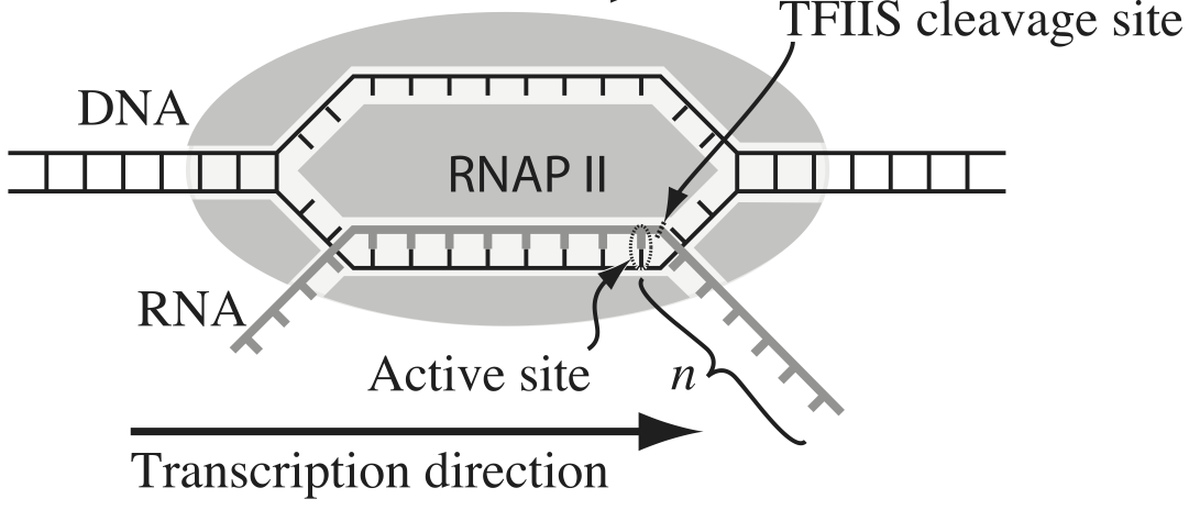
To escape these backtracks, a cleavage enzyme called TFIIS cleaves the bit on RNA hanging out of the front, and the RNAP can then go about its merry way.
Researchers have long debated how these backtracks are governed. Single molecule experiments can provide some much needed insight. The groups of Carlos Bustamante, Steve Block, and Stephan Grill, among others, have investigated the dynamics of RNAP in the absence of TFIIS. They can measure many individual backtracks and get statistics about how long the backtracks last.
One hypothesis is that the backtracks simply consist of diffusive-like motion along the DNA stand. That is to say, the polymerase can move forward or backward along the strand with equal probability once it is paused. This is a one-dimensional random walk. So, if we want to test this hypothesis, we would want to know how much time we should expect the RNAP to be in a backtrack so that we could compare to experiment.
So, we seek the probability density function of backtrack times, \(f(t_{bt})\), where \(t_{bt}\) is the time spent in the backtrack. We could solve this analytically, which requires some sophisticated mathematics. But, because we know how to draw random numbers, we can just compute this distribution directly using Monte Carlo simulation!
We start at \(x = 0\) at time \(t = 0\). We “flip a coin,” or choose a random number to decide whether we step left one base pair or right one base pair. The process of taking a step is modeled as a Poisson process, so the time needed to each step is Exponentially distributed. Depken, et al., report the average time for a step is about 0.5 seconds. So, once we decide which step to take, we draw a random number out of an Exponential distribution to determine how long it took to take the step.
We do this again and again, keeping track of how long we have been stepping and what the \(x\) position is. As soon as \(x\) becomes positive, we have existed the backtrack.
a) Write a function, that computes the amount of time it takes for a random walker (i.e., polymerase) starting at position \(x = 0\) to get to position \(x = +1\). It should return the total amount of time spent walking and, if you like, also the number of steps to take the walk.
b) Generate 10,000 of these backtracks in order to get enough samples out of \(f(t_\mathrm{bt})\). (If you are interested in a way to really speed up this calculation, you might want to try Numba.)
c) Generate an ECDF of your samples and plot the ECDF with the \(x\) axis on a logarithmic scale.
d) A probability distribution function that obeys a power law has the property
\begin{align} f(t_\mathrm{bt}) \propto t_\mathrm{bt}^{-\alpha-1} \end{align}
in some part of the distribution, usually for large \(t_\mathrm{bt}\). If this is the case, the cumulative distribution function is then
\begin{align} \mathrm{CDF}(t_\mathrm{bt}) \equiv F(t_\mathrm{bt})= \int_{-\infty}^{t_\mathrm{bt}} \mathrm{d}t_\mathrm{bt}'\,f(t_\mathrm{bt}') = 1 - \frac{c}{t_\mathrm{bt}^{\alpha}}, \end{align}
where \(c\) is some constant defined by the functional form of \(f(t_\mathrm{bt})\) for small \(t_\mathrm{bt}\) and the normalization condition. If \(F\) is our cumulative histogram, we can check for power law behavior by plotting the complementary cumulative distribution (CCDF), \(\bar{F}(t_\mathrm{bt}) = 1 - F(t_\mathrm{bt})\), versus \(t_\mathrm{bt}\). If a power law is in play, the plot will be linear on a log-log scale with a slope of \(-\alpha\).
Plot the complementary cumulative distribution function from your samples on a log-log plot. If it is linear, then the time to exit a backtrack is a power law.
e) By doing some mathematical heavy lifting, we know that, in the limit of large \(t_{bt}\),
\begin{align} f(t_{bt}) \propto t_{bt}^{-3/2}, \end{align}
so the plot you did in part (e) should have a slope of \(-1/2\) on a log-log plot of the empirical complementary cumulative distribution function. Is this what you see?
f) Under this model, does there exist a finite mean backtrack time? You should be able to answer this question with an analytical calculation, but a fun numerical experiment to test if your simulation is converging to a mean is to make a plot of the average of your first \(n\) backtrack times versus \(n\). If the mean exists, the mean you get by simulation should converge, as it does for a Normal distribution, shown below.
[2]:
hv.extension("bokeh")
# Get random samples
rg = np.random.default_rng()
x = rg.normal(0, 1, size=10000)
# Compute sequential means
n = np.arange(1, len(x)+1)
seq_mean = np.cumsum(x) / n
# Make plot
hv.Scatter(
data=(n, seq_mean),
kdims=['n'],
vdims=['mean']
).opts(
logx=True
)
[2]:
Notes: The theory to derive the probability distribution is involved. See, e.g., this. However, we were able to predict that we would see a great many short backtracks, and then see some very very long backtracks because of the power law distribution of backtrack times. We were able to do that just by doing a simple Monte Carlo simulation with “coin flips”. There are many problems where the theory is really hard, and deriving the distribution is currently impossible, or the probability distribution has such an ugly expression that we can’t really work with it. So, Monte Carlo methods are a powerful tool for generating predictions from simply-stated, but mathematically challenging, hypotheses.
Interestingly, many researchers thought (and maybe still do) there were two classes of backtracks: long and short. There may be, but the hypothesis that the backtrack is a random walk process is commensurate with seeing both very long and very short backtracks.