Building a model
[1]:
# Colab setup ------------------
import os, sys, subprocess
if "google.colab" in sys.modules:
    cmd = "pip install --upgrade iqplot bebi103 watermark"
    process = subprocess.Popen(cmd.split(), stdout=subprocess.PIPE, stderr=subprocess.PIPE)
    stdout, stderr = process.communicate()
    data_path = "https://s3.amazonaws.com/bebi103.caltech.edu/data/"
else:
    data_path = "../data/"
# ------------------------------

import numpy as np
import pandas as pd

import iqplot
import bebi103

import bokeh.io
bokeh.io.output_notebook()

import holoviews as hv
hv.extension('bokeh')

bebi103.hv.set_defaults()


As machine learning methods grow in power and prominence, and as data acquisition becomes more and more facile, we see more and more methods where a machine “learns” directly from data. Over a decade ago, Chris Anderson wrote an article entitled The End of Theory: The Data Deluge Makes the Scientific Method Obsolete in Wired Magazine. Anderson claimed that because we have access to large data sets, we no longer need the scientific method of testable hypotheses. Specifically, he says we do not need models, we can just use lots and lots of data to make predictions. This is absurd because if we just try to learn from data, we do not really learn anything fundamental about how nature works. If you are working for Netflix and trying to figure out what movies people want to watch, learning from data is fine. But if you’re a scientist and want to increase knowledge, you need models.
In this lesson, we introduce two competing models for how the size of mitotic spindles are set. I take the time to set up these models because it’s important; we should have a firm grasp on the theory behind our models.
What sets the size of mitotic spindles?
Matt Good and coworkers (Science, 2013) developed a microfluidic device where they could create droplets of cytoplasm extracted from Xenopus eggs and embryos, as shown the figure below (scale bar 20 µm; image taken from the paper).
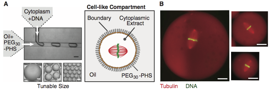
A remarkable property about Xenopus extract is that mitotic spindles spontaneously form; the extracted cytoplasm has all the ingredients to form them. This makes it an excellent model system for studying spindles. With their device, Good and his colleagues were able to study how the size of the cell affects the dimensions of the mitotic spindle; a simple, yet beautiful, question. The experiment is conceptually simple; they made the droplets and then measured their dimensions and the dimensions of the spindles using microscope images.
Let’s take a quick look at the result.
[2]:
hv.extension("bokeh")

df = pd.read_csv(os.path.join(data_path, 'good_invitro_droplet_data.csv'), comment='#')

hv.Scatter(
    data=df,
    kdims=['Droplet Diameter (um)'],
    vdims=['Spindle Length (um)']
)
[2]:
We now propose two models for how the droplet diameter affects the spindle length.
The spindles have an inherent length, independent of droplet diameter.
The length of spindles is determined by the total amount of tubulin available to make them.
Model 1: Spindle size is independent of droplet size
As a first model, we propose that the size of a mitotic spindle is inherent to the spindle itself. This means that the size of the spindle is independent of the size of the droplet or cell in which it resides. This would be the case, for example, if construction of the spindle involves length-sensing molecules, such as depolymerizing motor proteins. We define that set length as \(\phi\).
The statistical model
Not all spindles will be measured to be exactly \(\phi\) µm in length. Rather, there may be some variation about \(\phi\) due to natural variation and measurement error. So, we would expect measured length of spindle i to be
\begin{align} l_i = \phi + e_i, \end{align}
where \(e_i\) is the noise component of the \(i\)the datum.
So, we have a theoretical model for spindle length, \(l = \phi\), and to get a fully generative model, we need to model the errors \(e_i\). A reasonable model assumes
Each measured spindle’s length is independent of all others.
The variability in measured spindle length is Normally distributed.
With these assumptions, we can write the probability density function for \(l_i\) as
\begin{align} f(l_i ; \phi, \sigma) = \frac{1}{\sqrt{2\pi \sigma^2}}\,\exp\left[-\frac{(l_i - \phi)^2}{2\sigma^2}\right]. \end{align}
Since each measurement is independent, we can write the joint probability density function of the entire data set, which we will define as \(\mathbf{l} = \{l_1, l_2,\ldots\}\), consisting of \(n\) total measurements.
\begin{align} f(\mathbf{l} ; \phi, \sigma) = \prod_{i} f(l_i ; \phi, \sigma) = \frac{1}{(2\pi \sigma^2)^{n/2}}\,\exp\left[-\frac{1}{2\sigma^2}\sum_{i}(l_i - \phi)^2\right]. \end{align}
We can write this more succinctly, and perhaps more intuitively, as
\begin{align} l_i \sim \text{Norm}(\phi, \sigma) \;\;\forall i. \end{align}
We will generally write our models in this format, which is easier to parse and understand. Note that in writing this generative model, we have necessarily introduced another parameter, \(\sigma\), the standard deviation parametrizing the Normal distribution. So, we have two parameters in our model, \(\phi\) and \(\sigma\).
Model 2: Spindle length is set by total amount of tubulin
The cartoon model
The three key principles of this “cartoon” model are:
The total amount of tubulin in the droplet or cell is conserved.
The total length of polymerized microtubules is a function of the total tubulin concentration after assembly of the spindle. This results from the balances of microtubule polymerization rate with catastrophe frequencies.
The density of tubulin in the spindle is independent of droplet or cell volume.
The mathematical model
From these principles, we need to derive a mathematical model that will provide us with testable predictions. The derivation follows below (following the derivation presented in the paper), and you may read it if you are interested. Since our main focus here is building a statistical model, you can skip ahead to to the final equation, where we define a mathematical expression relating the spindle length, \(l\) to the droplet diameter, \(d\), which depends on two parameters, \(\gamma\) and \(\phi\). Nonetheless, it is important to see how a models such as this one is derived.
Principle 1 above (conservation of tubulin) implies
\begin{align} T_0 V_0 = T_1(V_0 - V_\mathrm{s}) + T_\mathrm{s}V_\mathrm{s}, \end{align}
where \(V_0\) is the volume of the droplet or cell, \(V_\mathrm{s}\) is the volume of the spindle, \(T_0\) is the total tubulin concentration (polymerized or not), \(T_1\) is the tubulin concentration in the cytoplasm after the the spindle has formed, and \(T_\mathrm{s}\) is the concentration of tubulin in the spindle. If we assume the spindle does not take up much of the total volume of the droplet or cell (\(V_0 \gg V_\mathrm{s}\), which is the case as we will see when we look at the data), we have
\begin{align} T_1 \approx T_0 - \frac{V_\mathrm{s}}{V_0}\,T_\mathrm{s}. \end{align}
The amount of tubulin in the spindle can we written in terms of the total length of polymerized microtubules, \(L_\mathrm{MT}\) as
\begin{align} T_s V_\mathrm{s} = \alpha L_\mathrm{MT}, \end{align}
where \(\alpha\) is the tubulin concentration per unit microtubule length. (We will see that it is unimportant, but from the known geometry of microtubules, \(\alpha \approx 2.7\) nmol/µm.)
We now formalize assumption 2 into a mathematical expression. Microtubule length should grow with increasing \(T_1\). There should also be a minimal threshold \(T_\mathrm{min}\) where polymerization stops. We therefore approximate the total microtubule length as a linear function,
\begin{align} L_\mathrm{MT} \approx \left\{\begin{array}{ccl} 0 & &T_1 \le T_\mathrm{min} \\ \beta(T_1 - T_\mathrm{min}) & & T_1 > T_\mathrm{min}. \end{array}\right. \end{align}
Because spindles form in Xenopus extract, \(T_0 > T_\mathrm{min}\), so there exists a \(T_1\) with \(T_\mathrm{min} < T_1 < T_0\). Thus, going forward, we are assured that \(T_1 > T_\mathrm{min}\). So, we have
\begin{align} V_\mathrm{s} \approx \alpha\beta\,\frac{T_1 - T_\mathrm{min}}{T_\mathrm{s}}. \end{align}
With insertion of our expression for \(T_1\), this becomes
\begin{align} V_{\mathrm{s}} \approx \alpha \beta\left(\frac{T_0 - T_\mathrm{min}}{T_\mathrm{s}} - \frac{V_\mathrm{s}}{V_0}\right). \end{align}
Solving for \(V_\mathrm{s}\), we have
\begin{align} V_\mathrm{s} \approx \frac{\alpha\beta}{1 + \alpha\beta/V_0}\,\frac{T_0 - T_\mathrm{min}}{T_\mathrm{s}} =\frac{V_0}{1 + V_0/\alpha\beta}\,\frac{T_0 - T_\mathrm{min}}{T_\mathrm{s}}. \end{align}
We approximate the shape of the spindle as a prolate spheroid with major axis length \(l\) and minor axis length \(w\), giving
\begin{align} V_\mathrm{s} = \frac{\pi}{6}\,l w^2 = \frac{\pi}{6}\,k^2 l^3, \end{align}
where \(k \equiv w/l\) is the aspect ratio of the spindle. We can now write an expression for the spindle length as
\begin{align} l \approx \left(\frac{6}{\pi k^2}\, \frac{T_0 - T_\mathrm{min}}{T_\mathrm{s}}\, \frac{V_0}{1+V_0/\alpha\beta}\right)^{\frac{1}{3}}. \end{align}
For small droplets, with \(V_0\ll \alpha \beta\), this becomes
\begin{align} l \approx \left(\frac{6}{\pi k^2}\, \frac{T_0 - T_\mathrm{min}}{T_\mathrm{s}}\, V_0\right)^{\frac{1}{3}} = \left(\frac{T_0 - T_\mathrm{min}}{k^2T_\mathrm{s}}\right)^{\frac{1}{3}}\,d, \end{align}
where \(d\) is the diameter of the spherical droplet or cell. So, we expect the spindle size to increase linearly with the droplet diameter for small droplets.
For large \(V_0\), the spindle size becomes independent of droplet size;
\begin{align} l \approx \left(\frac{6 \alpha \beta}{\pi k^2}\, \frac{T_0 - T_\mathrm{min}}{T_\mathrm{s}}\right)^{\frac{1}{3}}. \end{align}
Indentifiability of parameters
We measure the microtubule length \(l\) and droplet diameter \(d\) directly from the images. We can also measure the spindle aspect ratio \(k\) directly from the images. Thus, we have four unknown parameters, since we already know α ≈ 2.7 nmol/µm. The unknown parameters are:
parameter |
meaning |
|---|---|
\(\beta\) |
rate constant for MT growth |
\(T_0\) |
total tubulin concentration |
\(T_\mathrm{min}\) |
critical tubulin concentration for polymerization |
\(T_s\) |
tubulin concentration in the spindle |
We would like to determine all of these parameters. We could measure them all either in this experiment or in other experiments. We could measure the total tubulin concentration \(T_0\) by doing spectroscopic or other quantitative methods on the Xenopus extract. We can \(T_\mathrm{min}\) and \(T_s\) might be assessed by other in vitro assays, though these parameters may by strongly dependent on the conditions of the extract.
Importantly, though, the parameters only appear in combinations with each other in our theoretical model. Specifically, we can define two parameters,
\begin{align} \gamma &= \left(\frac{T_0-T_\mathrm{min}}{k^2T_\mathrm{s}}\right)^\frac{1}{3} \\ \phi &= \gamma\left(\frac{6\alpha\beta}{\pi}\right)^{\frac{1}{3}}. \end{align}
We can then rewrite the general model expression in terms of these parameters as
\begin{align} l(d) \approx \frac{\gamma d}{\left(1+(\gamma d/\phi)^3\right)^{\frac{1}{3}}}. \end{align}
If we tried to determine all four parameters from this experiment only, we would be in trouble. This experiment alone cannot distinguish all of the parameters. Rather, we can only distinguish two combinations of them, which we have defined as \(\gamma\) and \(\phi\). This is an issue of identifiability. We may not be able to distinguish all parameters in a given model, and it is important to think carefully before the analysis about which ones we can identify. Even with our work so far, we are not quite done with characterizing identifiability.
Visualizing the mathematical model
Let’s take a quick look at the mathematical model so we can see how the curve looks. It’s best to nondimensionalize the diameter by \(\phi\), giving
\begin{align} \frac{l(d)}{\phi} \approx \frac{\gamma d/\phi}{\left(1+(\gamma d/\phi)^3\right)^{\frac{1}{3}}}. \end{align}
So, we will plot \(l(/\phi\) versus \(d/\phi\), which means we choose units of length to be \(\phi\).
[3]:
hv.extension("bokeh")

def theor_spindle_length(gamma, d):
    """Compute spindle length using mathematical model"""
    return gamma * d / np.cbrt(1 + (gamma * d)**3)

d = np.linspace(0, 20, 200)

def plot_theor(gamma):
    return hv.Curve(
        data=(d, theor_spindle_length(gamma, d)),
        kdims=['d/φ'],
        vdims=['l/φ'],
        label=f'γ = {gamma}',
    ).opts(
        color=hv.Cycle(list(bokeh.palettes.Blues7[1:-1][::-1]))
    )

plots = [plot_theor(gamma) for gamma in [0.03, 0.1, 0.3, 0.7, 1.0]]

hv.Overlay(plots)
[3]:
The curve grows from zero to a plateau at \(l = \phi\), more rapidly for larger \(\gamma\). We can more carefully characterize the limiting behavior.
Limiting behavior
For large droplets, with \(d \gg \phi/\gamma\), the spindle size becomes independent of \(d\), with
\begin{align} l \approx \phi. \end{align}
Conversely, for \(d \ll \phi/\gamma\), the spindle length varies approximately linearly with diameter.
\begin{align} l(d) \approx \gamma\,d. \end{align}
Note that the expression for the linear regime gives bounds for \(\gamma\). Obviously, \(\gamma > 0\), lest we get negative spindle lengths. Because \(l \le d\), lest the spindle not fit in the droplet, we also have \(\gamma \le 1\).
Importantly, if the experiment is done in the regime where \(d\) is large (and we do not really know a priori how large that is since we do not know the parameters \(\phi\) and \(\gamma\)), we cannot tell the difference between the two models, since they are equivalent in that regime. Further, if the experiment is in this regime the model is unidentifiable because we cannot resolve \(\gamma\).
This sounds kind of dire, but this is actually a convenient fact. The second model is more complex, but it has the simpler model, model 1, as a limit. Thus, the two models are in fact commensurate with each other. Knowledge of how these limits work also enhances the experimental design. We should strive for small droplets. And perhaps most importantly, if we didn’t consider the second model, we might automatically assume that droplet size has nothing to do with spindle length if we simply did the experiment in larger droplets.
Generative model
We have a theoretical model relating the droplet diameter to the spindle length. Let us now build a generative model. For spindle, droplet pair i, we assume
\begin{align} l_i = \frac{\gamma d_i}{\left(1+(\gamma d/\phi)^3\right)^{\frac{1}{3}}} + e_i. \end{align}
We will assume that \(e_i\) is Normally distributed with variance \(\sigma^2\). This leads us to our statistical model.
\begin{align} &\mu_i = \frac{\gamma d_i}{\left(1+(\gamma d_i/\phi)^3\right)^{\frac{1}{3}}}, \\[1em] &l_i \sim \text{Norm}(\mu_i, \sigma) \;\forall i, \end{align}
which is equivalently stated as
\begin{align} l_i \sim \text{Norm}\left(\frac{\gamma d_i}{\left(1+(\gamma d_i/\phi)^3\right)^{\frac{1}{3}}}, \sigma\right) \;\forall i. \end{align}
Importantly, note that this model builds upon our first model. Generally, when doing modeling, it is a good idea to build more complex models on your initial baseline model such that the models are related to each other by limiting behavior. This gives you a continuum of model and a sound basis for making comparisons among models.
Note that we are assuming the droplet diameters are known. When we generate data sets for prior predictive checks, we will randomly generate them from about 20 µm to 200 µm, since this is the range achievable with the microfluidic device.
Checking model assumptions
In deriving the mathematical model, we made a series of assumptions. It is generally a good idea to check to see if assumptions in the mathematical modeling are realized in the experiment. If they are not, you may need to relax the assumptions and have a potentially more complicated model (which may suffer from identifiability issues). This underscores the interconnection between modeling and experimental design. You can allow for modeling assumptions and identifiability if you design your experimental parameters to meet the assumptions (e.g., choosing the appropriate range of droplet sizes).
Let’s do a quick verification that the droplet volume is indeed much larger than the spindle volume. Remember, the spindle volume for a prolate spheroid of length \(l\) and width \(w\) is \(V_\mathrm{s} = \pi l w^2 / 6\).
[4]:
# Compute spindle volume
spindle_volume = np.pi * df['Spindle Length (um)'] * df['Spindle Width (um)']**2 / 6

# Compute the ratio V_s / V_0 (taking care of units)
vol_ratio = spindle_volume / df['Droplet Volume (uL)'] * 1e-9

# Plot an ECDF of the results
bokeh.io.show(iqplot.ecdf(vol_ratio.values, x_axis_label='Vs/V0'))
We see that for pretty much all spindles that were measured, \(V_\mathrm{s} / V_0\) is small, so this is a sound assumption.
In setting up our model, we assumed that all spindles had the same aspect ratio. We can check this assumption because we have the data to do so available to us.
[5]:
# Compute the aspect ratio
k = df['Spindle Width (um)'] / df['Spindle Length (um)']

# Plot ECDF
bokeh.io.show(iqplot.ecdf(k.values, x_axis_label='k'))
The median aspect ratio is about 0.4, and we see spindle lengths about \(\pm 25\%\) of that. This could be significant variation. We may wish to update the model to account for nonconstant \(k\). Going forward, we will assume \(k\) is constant, but you may wish to perform the analysis in this and subsequent lessons with nonconstant \(k\) as an exercise.
Importantly, these checks of the model highlight the importance of checking your assumptions against your data. Always a good idea!
Computing environment
[6]:
%load_ext watermark
%watermark -v -p numpy,pandas,bokeh,holoviews,iqplot,bebi103,jupyterlab
CPython 3.8.5
IPython 7.19.0

numpy 1.19.2
pandas 1.1.3
bokeh 2.2.3
holoviews 1.13.5
iqplot 0.1.6
bebi103 0.1.1
jupyterlab 2.2.6