Introduction to data frames

Data set download

---

import numpy as np
import pandas as pd

---

Throughout your research career, you will undoubtedly need to handle data, possibly lots of data. Once in a usable form, you are empowered to rapidly make graphics and perform statistical inference. Tidy data is an important format and we will discuss that in subsequent sections of this lesson. In an ideal world, data sets would be stored in tidy format and be ready to use. The data comes in lots of formats, and you will spend much of your time wrangling the data to get it into a usable format. Wrangling is the topic of the next lesson; for now all data sets will be in tidy format from the get-go.

The data set

We will explore using Pandas with a real data set. We will use a data set published in Beattie, et al., Perceptual impairment in face identification with poor sleep, Royal Society Open Science, 3, 160321, 2016. In this paper, researchers used the Glasgow Facial Matching Test (GMFT) to investigate how sleep deprivation affects a subject’s ability to match faces, as well as the confidence the subject has in those matches. Briefly, the test works by having subjects look at a pair of faces. Two such pairs are shown below.

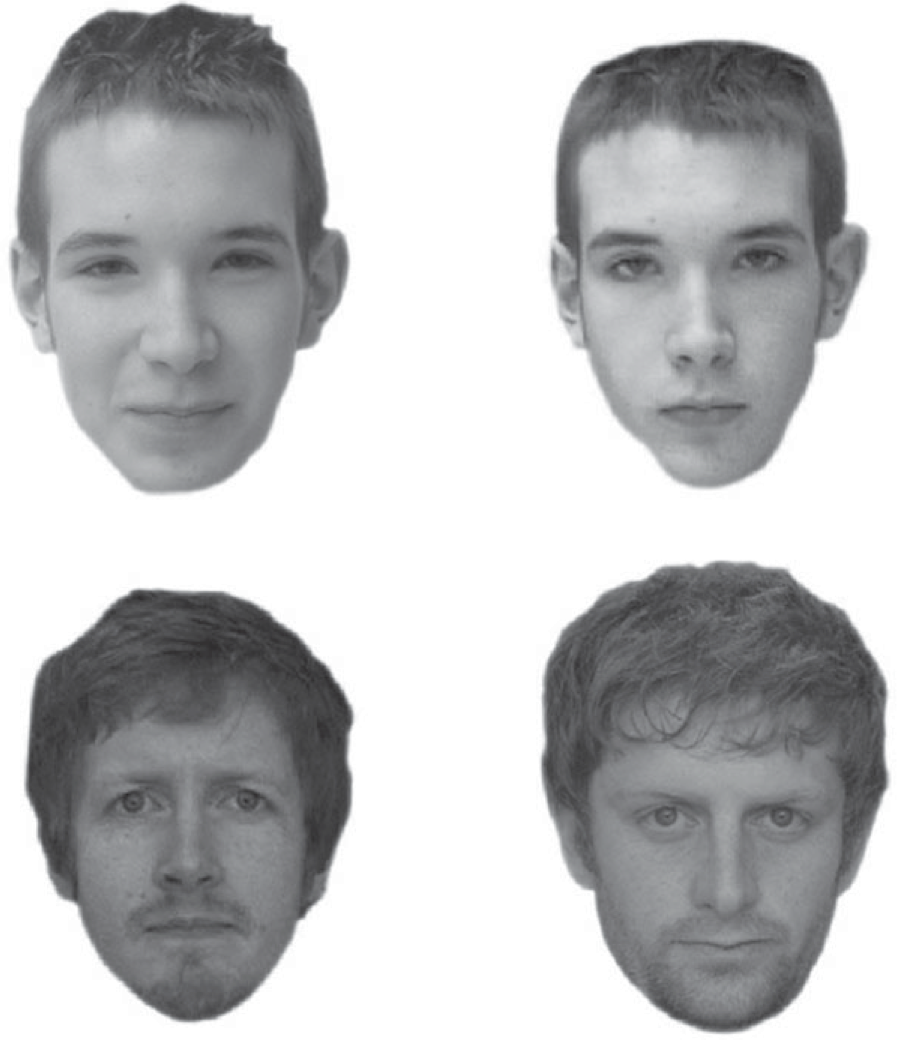
The top two pictures are the same person, the bottom two pictures are different people. For each pair of faces, the subject gets as much time as he or she needs and then says whether or not they are the same person. The subject then rates his or her confidence in the choice.

In this study, subjects also took surveys to determine properties about their sleep. The Sleep Condition Indicator (SCI) is a measure of insomnia disorder over the past month (scores of 16 and below indicate insomnia). The Pittsburgh Sleep Quality Index (PSQI) quantifies how well a subject sleeps in terms of interruptions, latency, etc. A higher score indicates poorer sleep. The Epworth Sleepiness Scale (ESS) assesses daytime drowsiness.

The data set can be downloaded here. The contents of this file were adapted from the Excel file posted on the public Dryad repository. (Note this: if you want other people to use and explore your data, make it publicly available.) I’ll say it more boldly.

If at all possible, share your data freely.

The data file is a CSV file, where CSV stands for comma-separated value. This is a text file that is easily read into data structures in many programming languages. You should generally always store your data in such a format, not necessarily CSV, but a format that is open, has a well-defined specification, and is readable in many contexts. Excel files do not meet these criteria. Neither do .mat files. There are other good ways to store data, such as JSON, but we will almost exclusively use CSV files in this class.

Let’s take a look at the CSV file. We will use the command line program head to look at the first 20 lines of the file.

!head ../data/gfmt_sleep.csv

participant number,gender,age,correct hit percentage,correct reject percentage,percent correct,confidence when correct hit,confidence incorrect hit,confidence correct reject,confidence incorrect reject,confidence when correct,confidence when incorrect,sci,psqi,ess
8,f,39,65,80,72.5,91,90,93,83.5,93,90,9,13,2
16,m,42,90,90,90,75.5,55.5,70.5,50,75,50,4,11,7
18,f,31,90,95,92.5,89.5,90,86,81,89,88,10,9,3
22,f,35,100,75,87.5,89.5,*,71,80,88,80,13,8,20
27,f,74,60,65,62.5,68.5,49,61,49,65,49,13,9,12
28,f,61,80,20,50,71,63,31,72.5,64.5,70.5,15,14,2
30,m,32,90,75,82.5,67,56.5,66,65,66,64,16,9,3
33,m,62,45,90,67.5,54,37,65,81.5,62,61,14,9,9
34,f,33,80,100,90,70.5,76.5,64.5,*,68,76.5,14,12,10

The first line contains the headers for each column. They are participant number, gender, age, etc. The data follow. There are two important things to note here. First, notice that the gender column has string data (m or f), while the rest of the data are numeric. Note also that there are some missing data, denoted by the *s in the file.

Given the file I/O skills you recently learned, you could write some functions to parse this file and extract the data you want. You can imagine that this might be kind of painful. However, if the file format is nice and clean, like we more or less have here, we can use pre-built tools to read in the data from the file and put it in a convenient data structure. This is one of the many uses of Pandas, a very powerful tool for handling data.

Pandas

Pandas is the primary tool in the Python ecosystem for handling data. Its primary object, the DataFrame is extremely useful in handling data. We will use Pandas to read in CSV (comma separated value) files and store the results in the very handy Pandas DataFrame. This incredibly flexible and powerful data structure will be a centerpiece in the rest of this course and beyond. In this lesson, we will learn about what a data frame is and how to use it.

Traditionally, Pandas is imported as pd, which we did in the first cell of this notebook.

Loading the data

Using pandas.read_csv() to read in data

We will use pd.read_csv() to load the data set. The data are stored in a data frame (data type DataFrame), which is one of the data types that makes Pandas so convenient for use in data analysis. Data frames offer mixed data types, including incomplete columns, and convenient slicing, among many, many other convenient features. We will use the data frame to look at the data, at the same time demonstrating some of the power of data frames. They are like spreadsheets, only a lot better.

df = pd.read_csv('../data/gfmt_sleep.csv', na_values='*')

Notice that we used the kwarg na_values=* to specify that entries marked with a * are missing. The resulting data frame is populated with a NaN, or not-a-number, wherever this character is present in the file. In this case, we want na_values='*'. So, let’s load in the data set.

If you check out the doc string for pd.read_csv(), you will see there are lots of options for reading in the data.

Exploring the DataFrame

Let’s jump right in and look at the contents of the DataFrame. We can look at the first several rows using the df.head() method.

# Look at the contents (first 5 rows)
df.head()

	participant number	gender	age	correct hit percentage	correct reject percentage	percent correct	confidence when correct hit	confidence incorrect hit	confidence correct reject	confidence incorrect reject	confidence when correct	confidence when incorrect	sci	psqi	ess
0	8	f	39	65	80	72.5	91.0	90.0	93.0	83.5	93.0	90.0	9	13	2
1	16	m	42	90	90	90.0	75.5	55.5	70.5	50.0	75.0	50.0	4	11	7
2	18	f	31	90	95	92.5	89.5	90.0	86.0	81.0	89.0	88.0	10	9	3
3	22	f	35	100	75	87.5	89.5	NaN	71.0	80.0	88.0	80.0	13	8	20
4	27	f	74	60	65	62.5	68.5	49.0	61.0	49.0	65.0	49.0	13	9	12

We see that the column headings were automatically assigned. Pandas also automatically defined the indices (names of the rows) as integers going up from zero. We could have defined the indices to be any of the columns of data, but since we did not specify anything for the index_col kwarg of pd.read_csv(), the default integer indexing is used.

Also note (in row 3) that the missing data are denoted as NaN.

Indexing data frames

The data frame is a convenient data structure for many reasons that will become clear as we start exploring. Let’s start by looking at how data frames are indexed. We could try to look at the first row like this:

df[0]

but that would be a mistake and we would get an error message (try it if you like). The problem is that we tried to index numerically by row. We index ``DataFrame``s, by columns. And there is no column that has the name 0 in this DataFrame, though there could be. Instead, a might want to look at the column with the percentage of correct face matching tasks. (To restrict the length of the output, I will use the .head() method to just show the first five rows. I’ll do this for much of the display of data frames and slices thereof in these lessons.)

df['percent correct'].head()

0    72.5
1    90.0
2    92.5
3    87.5
4    62.5
Name: percent correct, dtype: float64

This gave us the numbers we were after. Notice that when it was printed, the index of the rows came along with it. If we wanted to pull out a single percentage correct, say corresponding to index 4, we can do that.

df['percent correct'][4]

62.5

However, this is not the preferred way to do this. It is better to use ``.loc``. This give the location in the DataFrame we want.

df.loc[4, 'percent correct']

62.5

It is also important to note that row indices need not be integers. And you should not count on them being integers. In practice you will almost never use row indices, but rather use Boolean indexing. (Though see the caveat about speed, below.)

Boolean indexing of data frames

Let’s say I wanted the percent correct of participant number 42. I can use Boolean indexing to specify the row. Specifically, I want the row for which df['participant number'] == 42. You can essentially plop this syntax directly when using .loc.

df.loc[df['participant number'] == 42, 'percent correct']

54    85.0
Name: percent correct, dtype: float64

If I want to pull the whole record for that participant, I can use : for the column index.

df.loc[df['participant number'] == 42, :]

	participant number	gender	age	correct hit percentage	correct reject percentage	percent correct	confidence when correct hit	confidence incorrect hit	confidence correct reject	confidence incorrect reject	confidence when correct	confidence when incorrect	sci	psqi	ess
54	42	m	29	100	70	85.0	75.0	NaN	64.5	43.0	74.0	43.0	32	1	6

Notice that the index, 54, comes along for the ride, but we do not need it.

Now, let’s pull out all records of females under the age of 21. We can again use Boolean indexing, but we need to use an & operator, taken to mean logical AND. We did not cover this bitwise operator before, but the syntax is self-explanatory in the example below. Note that it is important that each Boolean operation you are doing is in parentheses because of the precedence of the operators involved. The other bitwise operators you may wish to use for Boolean indexing in data frames are | for OR and ~ for NOT.

df.loc[(df['age'] < 21) & (df['gender'] == 'f'), :]

	participant number	gender	age	correct hit percentage	correct reject percentage	percent correct	confidence when correct hit	confidence incorrect hit	confidence correct reject	confidence incorrect reject	confidence when correct	confidence when incorrect	sci	psqi	ess
27	3	f	16	70	80	75.0	70.0	57.0	54.0	53.0	57.0	54.5	23	1	3
29	5	f	18	90	100	95.0	76.5	83.0	80.0	NaN	80.0	83.0	21	7	5
66	58	f	16	85	85	85.0	55.0	30.0	50.0	40.0	52.5	35.0	29	2	11
79	72	f	18	80	75	77.5	67.5	51.5	66.0	57.0	67.0	53.0	29	4	6
88	85	f	18	85	85	85.0	93.0	92.0	91.0	89.0	91.5	91.0	25	4	21

We can do something even more complicated, like pull out all females under 30 who got more than 85% of the face matching tasks correct. The code is clearer if we set up our Boolean indexing first, as follows.

inds = (df['age'] < 30) & (df['gender'] == 'f') & (df['percent correct'] > 85)

# Take a look
inds.head()

0    False
1    False
2    False
3    False
4    False
dtype: bool

Notice that inds is an array (actually a Pandas Series, essentially a DataFrame with one column) of Trues and Falses. When we index with it using .loc, we get back rows where inds is True.

df.loc[inds, :]

	participant number	gender	age	correct hit percentage	correct reject percentage	percent correct	confidence when correct hit	confidence incorrect hit	confidence correct reject	confidence incorrect reject	confidence when correct	confidence when incorrect	sci	psqi	ess
22	93	f	28	100	75	87.5	89.5	NaN	67.0	60.0	80.0	60.0	16	7	4
29	5	f	18	90	100	95.0	76.5	83.0	80.0	NaN	80.0	83.0	21	7	5
30	6	f	28	95	80	87.5	100.0	85.0	94.0	61.0	99.0	65.0	19	7	12
33	10	f	25	100	100	100.0	90.0	NaN	85.0	NaN	90.0	NaN	17	10	11
56	44	f	21	85	90	87.5	66.0	29.0	70.0	29.0	67.0	29.0	26	7	18
58	48	f	23	90	85	87.5	67.0	47.0	69.0	40.0	67.0	40.0	18	6	8
60	51	f	24	85	95	90.0	97.0	41.0	74.0	73.0	83.0	55.5	29	1	7
75	67	f	25	100	100	100.0	61.5	NaN	58.5	NaN	60.5	NaN	28	8	9

Of interest in this exercise in Boolean indexing is that we never had to write a loop. To produce our indices, we could have done the following.

# Initialize array of Boolean indices
inds = [False] * len(df)

# Iterate over the rows of the DataFrame to check if the row should be included
for i, r in df.iterrows():
    if r['age'] < 30 and r['gender'] == 'f' and r['percent correct'] > 85:
        inds[i] = True

# Make our seleciton with Boolean indexing
df.loc[inds, :]

	participant number	gender	age	correct hit percentage	correct reject percentage	percent correct	confidence when correct hit	confidence incorrect hit	confidence correct reject	confidence incorrect reject	confidence when correct	confidence when incorrect	sci	psqi	ess
22	93	f	28	100	75	87.5	89.5	NaN	67.0	60.0	80.0	60.0	16	7	4
29	5	f	18	90	100	95.0	76.5	83.0	80.0	NaN	80.0	83.0	21	7	5
30	6	f	28	95	80	87.5	100.0	85.0	94.0	61.0	99.0	65.0	19	7	12
33	10	f	25	100	100	100.0	90.0	NaN	85.0	NaN	90.0	NaN	17	10	11
56	44	f	21	85	90	87.5	66.0	29.0	70.0	29.0	67.0	29.0	26	7	18
58	48	f	23	90	85	87.5	67.0	47.0	69.0	40.0	67.0	40.0	18	6	8
60	51	f	24	85	95	90.0	97.0	41.0	74.0	73.0	83.0	55.5	29	1	7
75	67	f	25	100	100	100.0	61.5	NaN	58.5	NaN	60.5	NaN	28	8	9

This feature, where the looping is done automatically on Pandas objects like DataFrames, is very powerful and saves us writing lots of lines of code. This example also showed how to use the iterrows() method of a DataFrame to iterate over the rows of a DataFrame. It is actually rare that you will need to do that, as we’ll show next when computing with DataFrames.

Calculating with data frames

Recall that a subject is said to suffer from insomnia if he or she has an SCI of 16 or below. We might like to add a column to the data frame that specifies whether or not the subject suffers from insomnia. We can conveniently compute with columns. This is done elementwise.

(df['sci'] <= 16).head()

0    True
1    True
2    True
3    True
4    True
Name: sci, dtype: bool

This tells use who is an insomniac. We can simply add this to the DataFrame.

# Add the column to the DataFrame
df['insomnia'] = df['sci'] <= 16

# Take a look
df.head()

	participant number	gender	age	correct hit percentage	correct reject percentage	percent correct	confidence when correct hit	confidence incorrect hit	confidence correct reject	confidence incorrect reject	confidence when correct	confidence when incorrect	sci	psqi	ess	insomnia
0	8	f	39	65	80	72.5	91.0	90.0	93.0	83.5	93.0	90.0	9	13	2	True
1	16	m	42	90	90	90.0	75.5	55.5	70.5	50.0	75.0	50.0	4	11	7	True
2	18	f	31	90	95	92.5	89.5	90.0	86.0	81.0	89.0	88.0	10	9	3	True
3	22	f	35	100	75	87.5	89.5	NaN	71.0	80.0	88.0	80.0	13	8	20	True
4	27	f	74	60	65	62.5	68.5	49.0	61.0	49.0	65.0	49.0	13	9	12	True

A note about vectorization

Notice how applying the <= operator to a Series resulted in elementwise application. This is called vectorization. It means that we do not have to write a for loop to do operations on the elements of a Series or other array-like object. Imagine if we had to do that with a for loop.

insomnia = []
for sci in df['sci']:
    insomnia.append(sci <= 16)

This is cumbersome. The vectorization allows for much more convenient calculation. Beyond that, the vectorized code is almost always faster when using Pandas and Numpy because the looping is done with compiled code under the hood. This can be done with many operators, including those you’ve already seen, like +, -, *, /, **, etc., just as with Numpy arrays.

Applying functions to Pandas objects

Remember when we saw the np.mean() function? We can compute with that as well. Let’s compare the mean percent correct for insomniacs versus those who are not.

print('Insomniacs:', np.mean(df.loc[df['insomnia'], 'percent correct']))
print('Control:   ', np.mean(df.loc[~df['insomnia'], 'percent correct']))

Insomniacs: 76.1
Control:    81.46103896103897

Notice that I used the ~ operator, which is a bit switcher. It changes all Trues to Falses and vice versa. In this case, it functions like NOT.

We will do a lot more computing with Pandas data frames as the course goes on. For our last demonstration in this lesson, we can quickly compute summary statistics about each column of a data frame using its describe() method.

df.describe()

	participant number	age	correct hit percentage	correct reject percentage	percent correct	confidence when correct hit	confidence incorrect hit	confidence correct reject	confidence incorrect reject	confidence when correct	confidence when incorrect	sci	psqi	ess
count	102.000000	102.000000	102.000000	102.000000	102.000000	102.000000	84.000000	102.000000	93.000000	102.000000	99.000000	102.000000	102.000000	102.000000
mean	52.049020	37.921569	83.088235	77.205882	80.147059	74.990196	58.565476	71.137255	61.220430	74.642157	61.979798	22.245098	5.274510	7.294118
std	30.020909	14.029450	15.091210	17.569854	12.047881	14.165916	19.560653	14.987479	17.671283	13.619725	15.921670	7.547128	3.404007	4.426715
min	1.000000	16.000000	35.000000	20.000000	40.000000	29.500000	7.000000	19.000000	17.000000	24.000000	24.500000	0.000000	0.000000	0.000000
25%	26.250000	26.500000	75.000000	70.000000	72.500000	66.000000	46.375000	64.625000	50.000000	66.000000	51.000000	17.000000	3.000000	4.000000
50%	52.500000	36.500000	90.000000	80.000000	83.750000	75.000000	56.250000	71.250000	61.000000	75.750000	61.500000	23.500000	5.000000	7.000000
75%	77.750000	45.000000	95.000000	90.000000	87.500000	86.500000	73.500000	80.000000	74.000000	82.375000	73.000000	29.000000	7.000000	10.000000
max	103.000000	74.000000	100.000000	100.000000	100.000000	100.000000	92.000000	100.000000	100.000000	100.000000	100.000000	32.000000	15.000000	21.000000

This gives us a data frame with summary statistics. Note that in this data frame, the row indices are not integers, but are the names of the summary statistics. If we wanted to extract the median value of each entry, we could do that with .loc.

df.describe().loc['50%', :]

participant number             52.50
age                            36.50
correct hit percentage         90.00
correct reject percentage      80.00
percent correct                83.75
confidence when correct hit    75.00
confidence incorrect hit       56.25
confidence correct reject      71.25
confidence incorrect reject    61.00
confidence when correct        75.75
confidence when incorrect      61.50
sci                            23.50
psqi                            5.00
ess                             7.00
Name: 50%, dtype: float64

Outputting a new CSV file

Now that we added the insomniac column, we might like to save our data frame as a new CSV that we can reload later. We use df.to_csv() for this with the index kwarg to ask Pandas not to explicitly write the indices to the file.

df.to_csv('gfmt_sleep_with_insomnia.csv', index=False)

Let’s take a look at what this file looks like.

!head gfmt_sleep_with_insomnia.csv

participant number,gender,age,correct hit percentage,correct reject percentage,percent correct,confidence when correct hit,confidence incorrect hit,confidence correct reject,confidence incorrect reject,confidence when correct,confidence when incorrect,sci,psqi,ess,insomnia
8,f,39,65,80,72.5,91.0,90.0,93.0,83.5,93.0,90.0,9,13,2,True
16,m,42,90,90,90.0,75.5,55.5,70.5,50.0,75.0,50.0,4,11,7,True
18,f,31,90,95,92.5,89.5,90.0,86.0,81.0,89.0,88.0,10,9,3,True
22,f,35,100,75,87.5,89.5,,71.0,80.0,88.0,80.0,13,8,20,True
27,f,74,60,65,62.5,68.5,49.0,61.0,49.0,65.0,49.0,13,9,12,True
28,f,61,80,20,50.0,71.0,63.0,31.0,72.5,64.5,70.5,15,14,2,True
30,m,32,90,75,82.5,67.0,56.5,66.0,65.0,66.0,64.0,16,9,3,True
33,m,62,45,90,67.5,54.0,37.0,65.0,81.5,62.0,61.0,14,9,9,True
34,f,33,80,100,90.0,70.5,76.5,64.5,,68.0,76.5,14,12,10,True

Very nice. Notice that by default Pandas leaves an empty field for NaNs, and we do not need the na_values kwarg when we load in this CSV file.

Slicing with iloc

Let’s say we wanted to consider only the males in the study. We can slice them out and put them in a new data frame (actually a view into the existing data frame df) using Boolean indexing.

df_male = df.loc[df['gender']=='m', :]

df_male.head()

	participant number	gender	age	correct hit percentage	correct reject percentage	percent correct	confidence when correct hit	confidence incorrect hit	confidence correct reject	confidence incorrect reject	confidence when correct	confidence when incorrect	sci	psqi	ess	insomnia
1	16	m	42	90	90	90.0	75.5	55.5	70.5	50.0	75.0	50.0	4	11	7	True
6	30	m	32	90	75	82.5	67.0	56.5	66.0	65.0	66.0	64.0	16	9	3	True
7	33	m	62	45	90	67.5	54.0	37.0	65.0	81.5	62.0	61.0	14	9	9	True
18	78	m	31	100	70	85.0	92.0	NaN	81.0	60.0	87.5	60.0	14	6	11	True
19	80	m	28	100	50	75.0	100.0	NaN	100.0	100.0	100.0	100.0	12	7	12	True

Note that the indices of the original data frame came along for the ride. The third row, for example, has index 7. This might seem counterintuitive, but it is actually a good idea. Remember, indices of data frames do not have to be integers!

If we do for some reason want to index by the order of the rows and columns in the data frame, we can use iloc.

# Using iloc enables indexing by the corresponding sequence of integers
df_male.iloc[3, 0]

78

While this works, I warn that you really should not need to use iloc. If you find yourself using it, remember that you are relying on the sorting of the data frame, which may not be relevant nor reliable. So, use ``iloc`` at your own risk, the consequences of which could be dire!

The one instance where I use iloc is when I don’t care which row I get, I just want a row, so I will use something like df.iloc[0, :].

Renaming columns

You may be annoyed with the rather lengthy syntax of access column names and wish to change them. Actually, you probably do not want to do this. Explicit is better than implicit! And furthermore, high level plotting libraries, as we will soon see, often automatically use column names for axis labels. So, let’s instead lengthen a column name. Say we keep forgetting what ESS stands for an want to rename the ess column to “Epworth Sleepiness Scale.”

Data frames have a nice rename method to do this. To rename the columns, we provide a dictionary where the keys are current column names and the corresponding values are the names we which to check them to. While we are at it, we will choose descriptive names for all three of the sleep quality indices.

# Make a dictionary to rename columns
rename_dict = {
    "ess": "Epworth Sleepiness Scale",
    "sci": "Sleep Condition Indicator",
    "psqi": "Pittsburgh Sleep Quality Index",
}

# Rename the columns
df = df.rename(columns=rename_dict)

df.head()

	participant number	gender	age	correct hit percentage	correct reject percentage	percent correct	confidence when correct hit	confidence incorrect hit	confidence correct reject	confidence incorrect reject	confidence when correct	confidence when incorrect	Sleep Condition Indicator	Pittsburgh Sleep Quality Index	Epworth Sleepiness Scale	insomnia
0	8	f	39	65	80	72.5	91.0	90.0	93.0	83.5	93.0	90.0	9	13	2	True
1	16	m	42	90	90	90.0	75.5	55.5	70.5	50.0	75.0	50.0	4	11	7	True
2	18	f	31	90	95	92.5	89.5	90.0	86.0	81.0	89.0	88.0	10	9	3	True
3	22	f	35	100	75	87.5	89.5	NaN	71.0	80.0	88.0	80.0	13	8	20	True
4	27	f	74	60	65	62.5	68.5	49.0	61.0	49.0	65.0	49.0	13	9	12	True

We can go on and on about indexing Pandas DataFrames, because there are many ways to do it. For much more on all of the clever ways you can access data and subsets thereof in DataFrames, see the Pandas docs on indexing.

A note on indexing and speed

As we have seen Boolean indexing is very convenient and fits nicely into a logical framework which allows us to extract data according to criteria we want. The trade-off is speed. Slicing by Boolean indexing is essentially doing a reverse lookup in a dictionary. We have to loop through all values to find keys that match. This is much slower than directly indexing. Compare the difference in speed for indexing the percent correct by participant number 42 by Boolean indexing versus direct indexing (it’s row 54).

print("Boolean indexing:")
%timeit df.loc[df['participant number'] == 42, 'percent correct']

print("\nDirect indexing:")
%timeit df.loc[54, 'percent correct']

Boolean indexing:
418 µs ± 3.84 µs per loop (mean ± std. dev. of 7 runs, 1000 loops each)

Direct indexing:
6.57 µs ± 30.7 ns per loop (mean ± std. dev. of 7 runs, 100000 loops each)

The speed difference is stark, differing be almost two orders of magnitude. For larger data sets, or for analyses that require repeated indexing, this speed consideration may be important.

Computing environment

%load_ext watermark

%watermark -v -p numpy,pandas,jupyterlab

CPython 3.7.4
IPython 7.1.1

numpy 1.17.2
pandas 0.24.2
jupyterlab 1.1.4