Plotting smooth curves

---

import numpy as np
import scipy.special

import bokeh.plotting
import bokeh.io
bokeh.io.output_notebook()

Loading BokehJS ...

---

Sometimes you want to plot smooth functions, as opposed to measured data like we have done so far. To do this, you can use Numpy and/or Scipy to generate arrays of values of smooth functions.

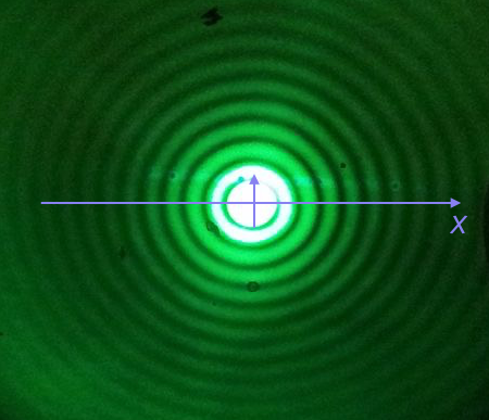
We will plot the Airy disk, which we encounter in biology when doing microscopy as the diffraction pattern of light passing through a pinhole. Here is a picture of the diffraction pattern from a laser (with the main peak overexposed).

The equation for the radial light intensity of an Airy disk is

\begin{align} \frac{I(x)}{I_0} = 4 \left(\frac{J_1(x)}{x}\right)^2, \end{align}

where \(I_0\) is the maximum intensity (the intensity at the center of the image) and \(x\) is the radial distance from the center. Here, \(J_1(x)\) is the first order Bessel function of the first kind. Yeesh. How do we plot that?

Fortunately, SciPy has lots of special functions available. Specifically, scipy.special.j1() computes exactly what we are after! We pass in a NumPy array that has the values of \(x\) we want to plot and then compute the \(y\)-values using the expression for the normalized intensity.

To plot a smooth curve, we use the np.linspace() function with lots of points. We then connect the points with straight lines, which to the eye look like a smooth curve. Let’s try it. We’ll use 400 points, which I find is a good rule of thumb for not-too-quickly-oscillating functions.

# The x-values we want
x = np.linspace(-15, 15, 400)

# The normalized intensity
norm_I = 4 * (scipy.special.j1(x) / x)**2

Now that we have the values we want to plot, we could construct a Pandas DataFrame to pass in as the source to p.line(). We do not need to take this extra step, though. If we instead leave source unspecified, and pass in NumPy arrays for x and y, Bokeh will directly use those in constructing the plot.

p = bokeh.plotting.figure(
    height=250,
    width=550,
    x_axis_label='x',
    y_axis_label='I(x)/I₀',
)

p.line(
    x=x,
    y=norm_I,
    line_join='bevel',
    line_width=2,
)

bokeh.io.show(p)

We could also plot dots (which doesn’t make sense here, but we’ll show it just to see who the line joining works to make a plot of a smooth function).

p.circle(
    x=x,
    y=norm_I,
    size=2,
    color='orange'
)

bokeh.io.show(p)

There is one detail I swept under the rug here. What happens if we compute the function for \(x = 0\)?

4 * (scipy.special.j1(0) / 0)**2

/Users/Justin/anaconda3/lib/python3.7/site-packages/ipykernel_launcher.py:1: RuntimeWarning: invalid value encountered in double_scalars
  """Entry point for launching an IPython kernel.

nan

We get a RuntimeWarning because we divided by zero. We know that

\begin{align} \lim_{x\to 0} \frac{J_1(x)}{x} = \frac{1}{2}, \end{align}

so we could write a new function that checks if \(x = 0\) and returns the appropriate limit for \(x = 0\). In the x array I constructed for the plot, we hopped over zero, so it was never evaluated. If we were being careful, we could write our own Airy function that deals with this.

def airy_disk(x):
    """Compute the Airy disk."""
    # Set up output array
    res = np.empty_like(x)

    # Where x is very close to zero (use np.isclose)
    near_zero = np.isclose(x, 0)

    # Compute values where x is close to zero
    res[near_zero] = 1.0

    # Everywhere else
    x_vals = x[~near_zero]
    res[~near_zero] = 4 * (scipy.special.j1(x_vals) / x_vals)**2

    return res

Computing environment

%load_ext watermark
%watermark -v -p numpy,scipy,bokeh,jupyterlab

CPython 3.7.4
IPython 7.1.1

numpy 1.17.2
scipy 1.3.1
bokeh 1.3.4
jupyterlab 1.1.4