R3. Time series and data smoothing

Dataset 1 download, Dataset 2 download

---

import numpy as np
import pandas as pd
import scipy.signal

import bebi103
import iqplot

import holoviews as hv
import holoviews.operation.datashader
hv.extension('bokeh')

import bokeh
bokeh.io.output_notebook()
bebi103.hv.set_defaults()

/Users/bois/opt/anaconda3/lib/python3.8/site-packages/arviz/__init__.py:317: UserWarning: Trying to register the cmap 'cet_gray' which already exists.
  register_cmap("cet_" + name, cmap=cmap)
/Users/bois/opt/anaconda3/lib/python3.8/site-packages/arviz/__init__.py:317: UserWarning: Trying to register the cmap 'cet_gray_r' which already exists.
  register_cmap("cet_" + name, cmap=cmap)

Loading BokehJS ...

---

Time Series with Holoviews

In lesson 4, we learned that Holoviews is a useful tool to group and overlay plots when we have different experimental conditions. Let’s practice this with time series data and multiple experimental groups.

The data were collected by Liana Merk, a student in the 2019 edition and TA in the 2020 edition of this course. She has seven strains of engineered E. coli that can respond to tetrathionate, a molecule is present in the gut during periods of inflammation. The engineered bacteria use a two-component system (TCS) to sense the external tetrathionate molecule, shown below.

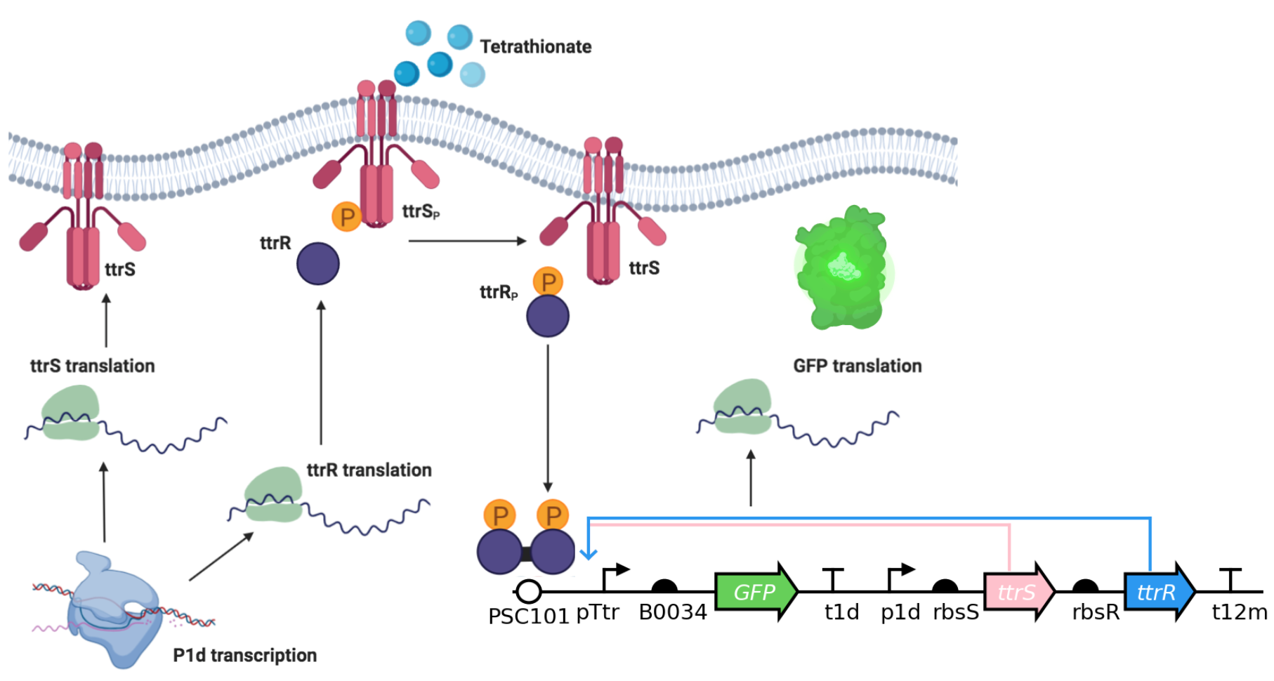
We can quantify activation of the circuit by measuring our fluorescent marker, GFP. In the given (tidy!) dataset, each a Biotek plate reader measured GFP fluorescence (Excitation: 483, Emission: 510, Gain 100), and optical density (absorbance at 700 nm). Let’s take a look at the dataframe.

df = pd.read_csv(os.path.join(data_path, "plate_reader.csv"))
df

	Sample	TTR_Concentration_mM	GFP/OD	Time_hr
0	LM13	0.0	12066.079295	0.033333
1	LM13	0.0	11153.526971	0.116667
2	LM13	0.0	10125.954198	0.200000
3	LM13	0.0	8760.942761	0.283333
4	LM13	0.0	7925.000000	0.366667
...	...	...	...	...
16123	CSH50	10.0	65506.702413	23.616667
16124	CSH50	10.0	66279.569892	23.700000
16125	CSH50	10.0	65306.451613	23.783333
16126	CSH50	10.0	65140.161725	23.866667
16127	CSH50	10.0	65892.183288	23.950000

16128 rows × 4 columns

We notice that we have already normalized fluorescence intensity to number of cells as best we can, by having a GFP/OD column. We have this measurement over time, given here in hours. In the sample column, we have each of the seven different engineered E. coli samples. The TTR_concentration_mM column represents how much tetrathionate we have for that given sample, ranging from 0 to 10 mM. We want to see how each of the samples responds to increasing tetrathionate concenration.

This is an exercise in using HoloViews to quickly make plots of these time series. Some notes about the code below:

1. When specifying a kdim or vdim, if you want its label in plots to be different than the column heading in the data frame, enter the kdim or vdim as a two-tuple, e.g., ("Time_hr", "time (hr)")).

2. To specify a set of colors, we use hv.Cycle(). The colors we will use are quantitative, since they are encoding for the TTR concentration, so we use a Viridis color map.bokeh.palettes.Viridis10 gives Viridis with ten levels. I often find that the extreme values on a color map are not the best for display, so I omit them, using instead the middle eight values.

3. If we place a legend outside of the plot area, it will take up space in the layout, resulting in extra unwanted whitespace. This is an issue that the HoloViews devs are aware of, and will likely be fixed in a later release. We therefore place the legend inside one of the plots. To do so, we need to change how it is displayed, which we do in HoloViews using the legend_opts kwarg in opts().

4. The cols() method of a HoloViews Layout enables specification of the number of columns in a layout.

hv.extension("bokeh")

plot_list = [
    hv.Curve(
        data=df.loc[df["Sample"] == sample],
        kdims=[("Time_hr", "time (hr)")],
        vdims=[ "GFP/OD", ("TTR_Concentration_mM", "[TTR] (mM)")],
    )
    .groupby("TTR_Concentration_mM")
    .opts(
        color=hv.Cycle(list(bokeh.palettes.Viridis10[1:-1])),
        frame_height=200,
        frame_width=350,
        title=f"Tetrathionate Response Curve: {sample}",
        # Only show legend on first plot
        show_legend=i == 0,
        line_width=3,
    )
    .overlay()
    .opts(
        legend_position="top_left",
        # Display legend horizontally
        legend_cols=True,
        # Format legend to fit
        legend_opts=dict(
            label_text_font_size="6pt",
            title_text_font_size="7pt",
            glyph_width=15,
            spacing=1,
            padding=5
        ),
    )
    for i, sample in enumerate(sorted(df["Sample"].unique()))
]

hv.Layout(plot_list).cols(2)

Great work! It seems like there are a couple samples that may have more circuit activation in response to tetrathionate. Let’s now look at some time series data and learn how to (be) smooth.

---

Time Series with Smoothing

We will perform some exploratory data analysis with a specific type of data, time series data, in which we have data of the form \((t, x(t))\), where \(t\) represents sequential time. There is a rich literature on time series analysis, and we will only dip our toe into the surface here.

We will focus on a few aspects that often come up in time series analysis in biology. First, we will learn how to filter signals. Then, we will work on techniques for extracting features out of a time trace. For this last challenge, we will use some ad hoc methods.

The data are from Markus Meister’s group from Dawna Bagherian and Kyu Lee, two students from the 2015 editions of this course. They put electrodes in the retinal cells of a mouse and measured voltage. From the time trace of voltage, they can detect and characterize spiking events. Our goal in this tutorial is to detect these events from a time trace of voltage from a mouse retinal cell and determine the probability distribution for inter-spike waiting times. This particular mouse had no stimuli; it was just held in constant light.

Prepping the data

We’ll start by loading in the data set, which you can download here. Pandas is really clever, and you do not need to unzip the file. The units of time are milliseconds and the units of the voltage are microvolts.

# Load in DataFrame
df = pd.read_csv(
    os.path.join(data_path, "retina_trace.zip"),
    comment="#",
    names=["t (ms)", "V (µV)"],
)

# Take a look
df.head()

	t (ms)	V (µV)
0	303.96	-18.44
1	304.00	0.94
2	304.04	-6.35
3	304.08	-14.38
4	304.12	-0.52

In previous datasets, each data point was independent, so the order they were stored in the dataframe didn’t affect our exploratory data analysis. With time series order matters, and plotting packages will rely on the order for generating lines between points, so we will also ensure the dataframe is ordered by time points.

df = df.sort_values(by="t (ms)")

It will be convenient to reset time to start at zero, so let’s subtract the minimum time. We’ll also convert our units to seconds.

# Start at zero
df["t (ms)"] -= df["t (ms)"].min()

# Convert to seconds
df["t (ms)"] /= 1000
df = df.rename(columns={"t (ms)": "t (s)"})

Let’s see how long the trace is.

print("n_samples =", len(df))
print(" max time =", df["t (s)"].max(), "s")

n_samples = 2682401
 max time = 107.296 s

Whew! Over 2 million samples over almost two minutes. Let’s get the sampling rate, and do a quick check to make sure it’s uniform. (By the way, these are good checks to do when validating data.)

# Get sampling rate from first two points
inter_sample_time = df["t (s)"][1] - df["t (s)"][0]
print("inter_sample_time =", inter_sample_time, "s")

# Check to make sure they are all the same
print("All the same?:", np.allclose(np.diff(df["t (s)"]), inter_sample_time))

inter_sample_time = 4.000000000002046e-05 s
All the same?: True

Good! So, let’s save our sampling rate in units of Hz.

sampling_freq =  1 / inter_sample_time

Exploring the trace

We want to get a quick look at the data. Because the trace is very long, we will have trouble viewing it with Bokeh because such a large number of data points are displayed graphically. To deal with large data sets like this, we can use DataShader. Datashader renders the trace as an image for each level of zoom so that the browser does not have to visualize all of the data points at once. (This only works in the Jupyter notebook, not in its HTML rendering.) You can read the Datashader docs for more information on how this works. We will discuss Datashader in much greater depth when we talk about overplotting.

hv.extension("bokeh")

hv.operation.datashader.datashade(
    hv.Curve(data=df, kdims=["t (s)"], vdims=["V (µV)"]), aggregator="any", cmap="#1f77b4",
).opts(
    frame_height=300, frame_width=625, show_grid=True,
)

For convenience, I’ll make another plot with only 20,000 data points that you can view in the HTML rendering of this notebook.

hv.extension("bokeh")

hv.Curve(
    data=df.iloc[10000:30000, :], kdims=["t (s)"], vdims=["V (µV)"]
).opts(
    frame_height=300,
    frame_width=625,
    show_grid=True,
)

In the zoomed out view, we can see spiking events as obvious drops in the voltage. When we zoom in, we can see what an individual spike looks like. We’ll reproduce it here.

hv.extension("bokeh")

inds = (0.675 < df["t (s)"]) & (df["t (s)"] < 0.69)

hv.Curve(
    data=df.loc[inds, :], kdims=["t (s)"], vdims=["V (µV)"]
).opts(
    frame_height=300,
    frame_width=625,
    show_grid=True,
)

The signal in the frequency domain

We are used to looking at time series data in the time domain, but this is only one way to look at it. Another way is in the frequency domain. We will not go into the mathematical details here, but talk very loosely to get a feel for what it means to represent data in the frequency domain. You can imagine that a signal can be represented by the sum of sine waves of different frequency. High frequency aspects of the signal oscillate rapidly, while low frequency aspects of the signal vary slowly in time. We can represent a signal by the magnitudes that each frequency contributes to the total signal. So, instead of plotting a signal versus \(t\), we can plot the magnitudes, or Fourier coefficients, of each frequency versus the frequency, \(f\). A plot like this is called a periodogram, and is useful to see what is present in the signal.

We can do much more with these magnitudes corresponding to frequencies. Say we wanted to filter out high frequency parts of the signal because they constitute noise. We could just go to the frequency domain, set the magnitudes for high frequencies to zero, and then go back to the time domain.

The Fourier transform is a useful mathematical tool to take us to the frequency domain and back, via the inverse Fourier transform. The fast Fourier transform, or FFT, is a very fast algorithm to do this, and it is implemented in NumPy and SciPy. Furthermore, the scipy.signal module has many convenient functions for filtering in the frequency domain. We will make use of a Butterworth filter, which is one of the simplest frequency domain filters available.

The periodogram

Let’s see what frequencies are present in our signal by computing the periodogram. We do this by getting the frequencies associated with the Fourier coefficients using np.fft.fftfreq() and then computing the power spectral density, which is the square of the magnitude of the Fourier coefficients. We can then plot the result. For reasons we will not get in to here, we will only consider positive frequencies, since the Fourier coefficients for the negative frequencies are symmetric. Note that we could generate the periodogram automatically using

f, psd = scipy.signal.periodogram(df['V (µV)'], fs=sampling_freq)

but this is much slower to compute, due to all the bells and whistles included in scipy.signal.

Computing an FFT for a long signal that does not have many prime factors is very inefficient. This data set has 2682401 time points, which has a prime factorization of 141179×19, so the performance of the FFT algorithm may be very slow. For the purposes of this periodogram, we will only consider the first 2097152 points, since this is a power of two. (I timed this a couple years ago, and computing the periodogram for the array of length 2097152 takes about 160 ms, and computing it for the array of length 2682401 takes 8.5 minutes! That’s a 3000-fold difference!).

hv.extension("bokeh")

# Truncated signal for faster calculation
max_ind = 2 ** (int(np.floor(np.log2(len(df)))))
V_trunc = df["V (µV)"].values[:max_ind]

# Determine frequencies
f = np.fft.fftfreq(len(V_trunc)) * sampling_freq

# Compute power spectral density
psd = np.abs(np.fft.fft(V_trunc)) ** 2 / len(V_trunc)

# Make into DataFrame to enable DataShaded viewing
df_psd = pd.DataFrame(data={"f (Hz)": f[f >= 0], "PSD": psd[f >= 0]})

# Make plot
hv.operation.datashader.datashade(
    hv.Curve(
        data=df_psd, kdims=["f (Hz)"], vdims=["PSD"]), aggregator="any", cmap="#1f77b4"
).opts(
    frame_height=300, frame_width=625, show_grid=True
)

Note that we have frequencies up to 12,500 Hz. This is the Nyquist frequency, half the sampling frequency, which is the highest frequency that can be coded at a given sampling rate (in our case, 25,000 Hz).

There is a big peak at 8000 Hz, which corresponds to the dominant frequency in the signal. This is high-frequency noise, but it is important to keep these frequencies because the signal in spikes undergoes a rapid change in just a fraction of a millisecond. So, we probably want to keep the high frequencies.

The very low frequency peak at \(f = 0\) corresponds to the constant, or DC, signal. That obviously also does not include spikes. There is also some low frequency oscillation, which are clearly not related to spiking. If we want to detect spikes by setting a threshold voltage, though, it is important to filter out these low frequency variations.

As we saw from looking at the plots, a spike occurs over about 10 or 20 ms, which would be captured by sampling at about 200 Hz (2/0.01 s, according to the Nyquist sampling theorem). So, to make sure we get good resolution on the spikes, we should be sure not to filter out frequencies that are too close to 100 Hz.

Butterworth filter: a frequency filter

There are lots and lots of filters available, but we will use a simple Butterworth filter. We won’t go into the theory of filters, transfer functions, etc., here, but will get a graphical idea of how a Butterworth filter works. A Butterworth filter is a band pass filter, meaning that it lets certain bands of frequency “pass” and be included in the filtered signal. We want to construct a highpass filter because we just want to filter out the low frequencies.

We construct a Butterworth filter using scipy.signal.butter(). This function returns coefficients on polynomials for the numerator and denominator of a Butterworth filter, which you can read about on the Wikipedia page. We have to specify the order of the polynomials (we’ll use third order) and the cutoff frequency, which defines the frequency below which modes are cut off. The cutoff frequency has to be in units of the Nyquist frequency. We will put our cutoff at 50 Hz.

# Compute Nyquist frequency
nyquist_freq = sampling_freq / 2

# Design a butterworth filter
b, a = scipy.signal.butter(3, 100 / nyquist_freq, btype="high")

Let’s look at what frequencies get through this filter (the so-called frequency response). We can get the frequencies (in units of \(\pi/f_\text{Nyquist}\), or radians/sample) and the the response using scipy.signal.freqz().

hv.extension("bokeh")

# Get frequency response curve
w, h = scipy.signal.freqz(b, a, worN=2000)

# Make plot
hv.Curve(
    data=((nyquist_freq / np.pi) * w, abs(h)), kdims=["freq. (Hz)"], vdims=["response"],
).opts(
    frame_height=250,
    frame_width=400,
    logx=True,
    padding=0.05,
    show_grid=True,
    xlim=(10, 1e4),
)

So, we will block out frequencies below about 50 Hz and let high frequencies pass through. Let’s filter the voltages and look at the result. It’s easiest to see how the filter worked if we again just look at a subset of the whole signal.

hv.extension("bokeh")

# Filter data
df["V filtered (µV)"] = scipy.signal.lfilter(b, a, df["V (µV)"])

# Plot the result, overlaying filtered and unfiltered
curves = [
    hv.Curve(
        data=df.iloc[10000:30000, :], kdims=["t (s)"], vdims=V, label=filtered,
    ).opts(
        alpha=0.5,
        frame_height=300,
        frame_width=575,
        show_grid=True,
    )
    for filtered, V in zip(["unfiltered", "filtered"], ["V (µV)", "V filtered (µV)"])
]

hv.Overlay(curves)

The filtering did a good job of limited longer time scale variations while keeping the spikes intact. The spikes are a bit shorter, since there will always be some attenuation when you filter.

Finding the spikes

We’ll now use our filtered trace to locate the spikes. Our goal is to find the spikes, store a neighborhood around the spike, and then find the position of the spike to sub-sampling accuracy.

Locating spikes

To locate the spikes, we will search for places where the signal dips below a threshold and then rises up above it again. This will mark boundaries of the spike, and we will then keep half a millisecond of samples on the left side of the threshold crossing and 2 milliseconds on the right.

# Threshold below which spike has to drop (in µV)
thresh = -40

# Amount of time in seconds to keep on either side of spike
time_window_left = 0.0005
time_window_right = 0.002

# Number of samples to keep on either side of spike
n_window_left = int(time_window_left * sampling_freq)
n_window_right = int(time_window_right * sampling_freq)

# DataFrame to store spikes
df_spike = pd.DataFrame(columns=["spike", "t (s)", "V (µV)"])

# Use a NumPy array for speed in looping
V = df["V filtered (µV)"].values

# Initialize while loop
i = 1
spike = 0
while i < len(df):
    if V[i] < thresh:
        # Found a spike, get crossings
        cross_1 = i
        while V[i] < thresh:
            i += 1
        cross_2 = i

        # Store perintent quantities in DataFrame
        t_in = df["t (s)"][cross_1 - n_window_left : cross_2 + n_window_right]
        V_in = df["V (µV)"][cross_1 - n_window_left : cross_2 + n_window_right]
        data = {
            "t (s)": t_in,
            "V (µV)": V_in,
            "spike": spike * np.ones_like(t_in, dtype=int),
        }
        df_add = pd.DataFrame(data)
        df_spike = pd.concat((df_spike, df_add), sort=True)

        spike += 1

    i += 1

Now that we have found the spikes, let’s plot them all on top of each other to ascertain their shape. First, we should make a set of time points to plot them all on top of each other.

df_spike["relative time (s)"] = df_spike.groupby("spike")["t (s)"].transform(
    lambda x: np.arange(len(x)) / sampling_freq
)

Now we can make the plots.

hv.extension("bokeh")

hv.Curve(
    data=df_spike, kdims=["relative time (s)"], vdims=["V (µV)", "spike"]
).groupby(
    "spike"
).opts(
    alpha=0.05,
    color="#1f77b4",
    frame_height=300,
    frame_width=575,
    line_width=1,
    show_grid=True,
).overlay(
)

A smooth interpolant for the spike potential

We would like to describe the spike with a smooth function. In doing this, we can estimate the location of the bottom of the spike to greater accuracy than dictated by the sampling rate. We call a smooth curve that passes through the noisy data and interpolant.

Let’s look at a single spike as we develop the interpolant.

hv.extension("bokeh")

# Pull out 0th spike
spike = 0
df_0 = df_spike.loc[df_spike["spike"] == spike, :]

# Plot the spike
def base_spike_plot():
    line_plot = hv.Curve(
        data=df_0, kdims=["t (s)"], vdims=["V (µV)"]
    ).opts(
        frame_height=300,
        frame_width=575,
        color=bebi103.hv.default_categorical_cmap[0],
        line_width=1,
        padding=0.05,
        show_grid=True,
    )

    scatter_plot = hv.Scatter(data=df_0, kdims=["t (s)"], vdims=["V (µV)"]).opts(
        color=bebi103.hv.default_categorical_cmap[0], size=5,
    )

    return line_plot * scatter_plot


base_spike_plot()

We will consider several ways to get a smooth interpolant.

Smoothing with basis functions (splines)

A function \(f(x)\) (or data) can generally be written as an expansion of \(M\) orthogonal basis functions \(h_m\), such that

\begin{align} f(x) = \sum_{m=1}^M \beta_m\,h_m(x), \end{align}

where \(\beta_m\) are coefficients. Examples of basis functions you may be familiar with are sines/cosines (used to construct a Fourier series), Legendre polynomials, spherical harmonics, etc. The idea behind smoothing with basis functions is to control the complexity of \(f(x)\) by restricting the number of basis functions or selecting certain basis functions to use. This restricted \(f(x)\), being less complex than the data, is smoother.

A commonly used set of basis function are cubic polynomials. An approximation of this procedure is called a spline. If we have \(k\) joining points of cubic functions (called knots), the data are represented with \(k\) basis functions.

The scipy.interpolate module has spline tools. Importantly, it selects the number of knots to use until a smoothing condition is met. This condition is defined by

\begin{align} \sum_{i\in D} \left[w_i(y_i - \hat{y}(x_i))\right]^2 \le s, \end{align}

where \(w_i\) is the weight we wish to assign to data point \(i\), and \(\hat{y}(x_i)\) is the smoothed function at \(x_i\). We will take all \(w_i\)’s to be equal in our analysis. A good rule of thumb is to choose

\begin{align} s = f\sum_{i\in D} y_i^2, \end{align}

where \(f\) is roughly the fractional difference between the rough and smooth curves.

hv.extension("bokeh")

# Determine smoothing factor from rule of thumb (use f = 0.05)
smooth_factor = 0.05 * (df_0["V (µV)"] ** 2).sum()

# Set up an scipy.interpolate.UnivariateSpline instance
ts = df_0["t (s)"].values
Vs = df_0["V (µV)"].values
spl = scipy.interpolate.UnivariateSpline(ts, Vs, s=smooth_factor)

# spl is now a callable function
ts_spline = np.linspace(ts[0], ts[-1], 400)
Vs_spline = spl(ts_spline)

# Plot results
base_spike_plot() * hv.Curve(data=(ts_spline, Vs_spline)).opts(
    color="#ff7f0e", line_width=2
)

Perhaps we chose our smoothing factor to be too small. But a better explanation for the windy path of the spline curve is that the spike is highly localized and then imposes a large variation on the data. It might be better to only fit a spline in the close neighborhood of the spike.

hv.extension("bokeh")

minind = np.argmin(Vs)
ts_short = ts[minind - 7 : minind + 7]
Vs_short = Vs[minind - 7 : minind + 7]

smooth_factor = 0.05 * (Vs_short ** 2).sum()
spl = scipy.interpolate.UnivariateSpline(ts_short, Vs_short, s=smooth_factor)
ts_spline = np.linspace(ts_short[0], ts_short[-1], 400)
Vs_spline = spl(ts_spline)

# Plot results
base_spike_plot() * hv.Curve(data=(ts_spline, Vs_spline)).opts(
    color="#ff7f0e", line_width=2
)

Kernel-based smoothing

Another option for smoothing is a kernel-based method. We will use a Nadaraya-Watson kernel estimator, which is essentially a weighted average of the data points.

When we have a high sampling rate, the extra fine resolution often just gives the noise. We could do a sliding average over the data. I will write this process concretely. For ease of notation, we arrange our data points in time, i.e., index \(i+1\) follows \(i\) in time, with a total of \(n\) data points. For data point \((x_i, y_i)\), we get a smoothed value \(\hat{x}_i\) by

\begin{align} \hat{y}(x_0) = \frac{\sum_{i=1}^n K_\lambda(x_0, x_i)\, y_i}{\sum_{i=1}^n K_\lambda(x_0,x_i)} \end{align}

where \(K_\lambda(x_0, x_i)\) is the kernel, or weight. If we took each data point to be the mean of itself and its 10 nearest-neighbors, we would have (neglecting end effects)

\begin{align} K_\lambda(x_j, x_i) = \left\{\begin{array}{cl} \frac{1}{11} & \left|i - j\right| \le 5 \\[1mm] 0 & \text{otherwise}. \end{array} \right. \end{align}

Commonly used Kernels are the Epanechnikov quadratic kernel, the tri-cube kernel, and the Gaussian kernel. We can write them generically as

\begin{align} K_\lambda(x_0, x_i) &= D\left(\frac{\left|x_i-x_0\right|}{\lambda}\right) \equiv D(t), \\[1mm] \text{where } t &= \frac{\left|x_i-x_0\right|}{\lambda}. \end{align}

These kernels are

\begin{align} \text{Epanechnikov:}\;\;\;\;\; D &= \left\{\begin{array}{cl} \frac{3}{4}\left(1 - t^2\right) & |t| \le 1 \\[1mm] 0 & \text{otherwise} \end{array}\right. \\[5mm] \text{tri-cube:}\;\;\;\;\;D&=\left\{\begin{array}{cl} \left(1 - \left|t\right|^3\right)^3 & |t| \le 1 \\[1mm] 0 & \text{otherwise} \end{array}\right. \\[5mm] \text{Gaussian:}\;\;\;\;\;D &= \mathrm{e}^{-t^2}. \end{align}

Let’s code up functions for these kernels.

# Define our kernels
def epan_kernel(t):
    """
    Epanechnikov kernel.
    """
    return np.logical_and(t > -1.0, t < 1.0) * 3.0 * (1.0 - t ** 2) / 4.0


def tri_cube_kernel(t):
    """
    Tri-cube kernel.
    """
    return np.logical_and(t > -1.0, t < 1.0) * (1.0 - abs(t ** 3)) ** 3


def gauss_kernel(t):
    """
    Gaussian kernel.
    """
    return np.exp(-(t ** 2) / 2.0)

Now we can compare the respective kernels to get a feel for how the averaging goes.

hv.extension("bokeh")

# Set up time points
t = np.linspace(-4.0, 4.0, 200)
dt = t[1] - t[0]

# Compute unnormalized kernels
K_epan = epan_kernel(t)
K_tri_cube = tri_cube_kernel(t)
K_gauss = gauss_kernel(t)

# Adjust to approximately integrate to unity for ease of comparison
K_epan /= K_epan.sum() * dt
K_tri_cube /= K_tri_cube.sum() * dt
K_gauss /= K_gauss.sum() * dt

# Plot kernels; easier in base BOkeh
p = bokeh.plotting.figure(
    plot_height=300,
    plot_width=450,
    x_axis_label="t = |x-x0|/λ",
    y_axis_label="K(x0, x)",
)
p.line(t, K_epan, color="#ff7f0e", line_width=2, legend_label="Epanechnikov")
p.line(t, K_tri_cube, color="#2ca02c", line_width=2, legend_label="Tri-cube")
p.line(t, K_gauss, color="#9467bd", line_width=2, legend_label="Gaussian")
bokeh.io.show(p)

From the scale of the \(x\)-axis in this plot, we see that the parameter \(\lambda\) sets the width of the smoothing kernel. The bigger \(\lambda\) is, the stronger the smoothing and the more fine detail will be averaged over. For this reason, \(\lambda\) is sometimes called the bandwidth of the kernel. The Gaussian kernel is broad and has no cutoff like the Epanechnikov or tri-cube kernels. If therefore uses all of the data points.

We will now write a function to give the smoothed value of a function for a given kernel using Nadaraya-Watson.

def nw_kernel_smooth(x_0, x, y, kernel_fun, lam):
    """
    Gives smoothed data at points x_0 using a Nadaraya-Watson kernel
    estimator.  The data points are given by NumPy arrays x, y.

    kernel_fun must be of the form
        kernel_fun(t),
    where t = |x - x_0| / lam

    This is not a fast way to do it, but it simply implemented!
    """

    # Function to give estimate of smoothed curve at single point.
    def single_point_estimate(x_0_single):
        """
        Estimate at a single point x_0_single.
        """
        t = np.abs(x_0_single - x) / lam
        return np.dot(kernel_fun(t), y) / kernel_fun(t).sum()

    # If we only want an estimate at a single data point
    if np.isscalar(x_0):
        return single_point_estimate(x_0)
    else:  # Get estimate at all points
        return np.array([single_point_estimate(x) for x in x_0])

All right, we’re all set. Let’s try applying some kernels to our spike

hv.extension("bokeh")

# Specify time points
ts_kernel = np.linspace(ts[0], ts[-1], 400)

# Averaging window (0.2 ms)
lam = 0.0002

# Compute smooth curves with kernel
Vs_epan = nw_kernel_smooth(ts_kernel, ts, Vs, epan_kernel, lam)
Vs_tri_cube = nw_kernel_smooth(ts_kernel, ts, Vs, tri_cube_kernel, lam)
Vs_gauss = nw_kernel_smooth(ts_kernel, ts, Vs, gauss_kernel, lam)

# Plot results
plot = (
    base_spike_plot()
    * hv.Curve((ts_kernel, Vs_epan), label="Epanechnikov").opts(
        color="#ff7f0e", line_width=2
    )
    * hv.Curve((ts_kernel, Vs_tri_cube), label="Tri-cube").opts(
        color="#2ca02c", line_width=2
    )
    * hv.Curve((ts_kernel, Vs_gauss), label="Gaussian").opts(
        color="#9467bd", line_width=2
    )
)

plot.opts(legend_position="bottom_right")

All of these dull the spike. In fact, this is generally what you will find with smoothing methods.

The simple option

Why don’t we just fit a parabola to the bottom three points and then compute the minimum that way? If we approximate \(V(t) = at^2 + bt + c\) at the bottom of the spike, the minimum is at \(t = -b/2a\). We can do this easily using np.polyfit().

hv.extension("bokeh")

# Find minimum by fitting polynomial
minind = np.argmin(Vs)
V_vals = Vs[minind - 1 : minind + 2]
t_vals = ts[minind - 1 : minind + 2]
a, b, c = np.polyfit(t_vals, V_vals, 2)
t_min = -b / 2 / a

# Plot the result
plot * hv.Scatter((t_min, a * t_min ** 2 + b * t_min + c)).opts(
    size=16, color="#d62728", marker="diamond"
).opts(legend_position="bottom_right")

So, we’ll write a quick function to give our minimum.

def local_min(x, y):
    """
    Locally approximate minimum as quadratic
    and return location of minimum.
    """
    minind = np.argmin(y)
    y_vals = y[minind - 1 : minind + 2]
    x_vals = x[minind - 1 : minind + 2]
    a, b, c = np.polyfit(x_vals, y_vals, 2)

    return -b / 2 / a

Distribution of spike spacing

We’ll now compute the position of all spikes using the local_min function.

# Array to hold spike positions
spikes = np.empty(len(df_spike["spike"].unique()))

# Compute spike positions
for i, spike in enumerate(df_spike["spike"].unique()):
    inds = df_spike["spike"] == spike
    spikes[i] = local_min(
        df_spike["t (s)"][inds].values, df_spike["V (µV)"][inds].values
    )

# Compute interspike times
interspike_times = np.diff(spikes)

Now that we have the interspike times, we can plot their distribution.

# Make ECDF
p = iqplot.ecdf(
    data=interspike_times, q="interspike time (s)", x_axis_type="log", x_range=(4e-3, 5)
)
bokeh.io.show(p)

The distribution has a long tail. Many spikes occur in close to each other, and then there are long periods of quiescence. You could try various models to describe and parametrize this behavior, but I leave that as an enrichment exercise for you if you are interested.

This lesson was written by Justin Bois and added to by Sanjana Kulkarni and Liana Merk.

Computing environment

%load_ext watermark
%watermark -v -p numpy,scipy,pandas,bokeh,holoviews,datashader,iqplot,bebi103,jupyterlab

Python implementation: CPython
Python version       : 3.8.12
IPython version      : 7.27.0

numpy     : 1.21.2
scipy     : 1.7.1
pandas    : 1.3.3
bokeh     : 2.3.3
holoviews : 1.14.6
datashader: 0.13.0
iqplot    : 0.2.3
bebi103   : 0.1.8
jupyterlab: 3.1.7