R4. Manipulating data frames
This recitation was written by Sanjana Kulkarni with edits by Justin Bois.
[2]:
import string
import numpy as np
import pandas as pd
import scipy.optimize
import holoviews as hv
hv.extension("bokeh")
import bebi103
bebi103.hv.set_defaults()


/Users/bois/opt/anaconda3/lib/python3.8/site-packages/arviz/__init__.py:317: UserWarning: Trying to register the cmap 'cet_gray' which already exists.
register_cmap("cet_" + name, cmap=cmap)
/Users/bois/opt/anaconda3/lib/python3.8/site-packages/arviz/__init__.py:317: UserWarning: Trying to register the cmap 'cet_gray_r' which already exists.
register_cmap("cet_" + name, cmap=cmap)
Data from Plate Readers
In this recitation, we will practice some of the reshaping techniques you have been using in your homework with another example of 96-well plate reader data. Plate readers generally output Excel files, after which the data is tediously copy-pasted into Prism (or another Excel file) for plotting and analysis. We will use various Python functions to manipulate our data into tidy format and analyze them. You can download the data files here:
https://s3.amazonaws.com/bebi103.caltech.edu/data/20200117-1.xlsx
https://s3.amazonaws.com/bebi103.caltech.edu/data/20200117-2.xlsx
https://s3.amazonaws.com/bebi103.caltech.edu/data/20200117-3.xlsx
https://s3.amazonaws.com/bebi103.caltech.edu/data/20200117-4.xlsx
https://s3.amazonaws.com/bebi103.caltech.edu/data/20200117-5.xlsx
This data was collected by Sanjana Kulkarni and is an example of an enzyme-linked immunosorbance assay (ELISA). This assay measures the relative binding affinities between protein pairs, such as antibodies and the antigens to which they bind. The antigen is one of the surface glycoproteins of hepatitis C virus, and the antibodies are broadly neutralizing antibodies (bNAbs) isolated from hepatitis C virus patients. Stronger binding interactions result in higher observable fluorescence.
The plate reader measures absorbance at 450 nm because the chromogenic substrate produces a yellow-ish color when it is protonated by a strong acid. As in the homework, we are dealing with data in a 96-well format. Below is some other important information about the plate set up (with a diagram because a picture is worth a thousand words):
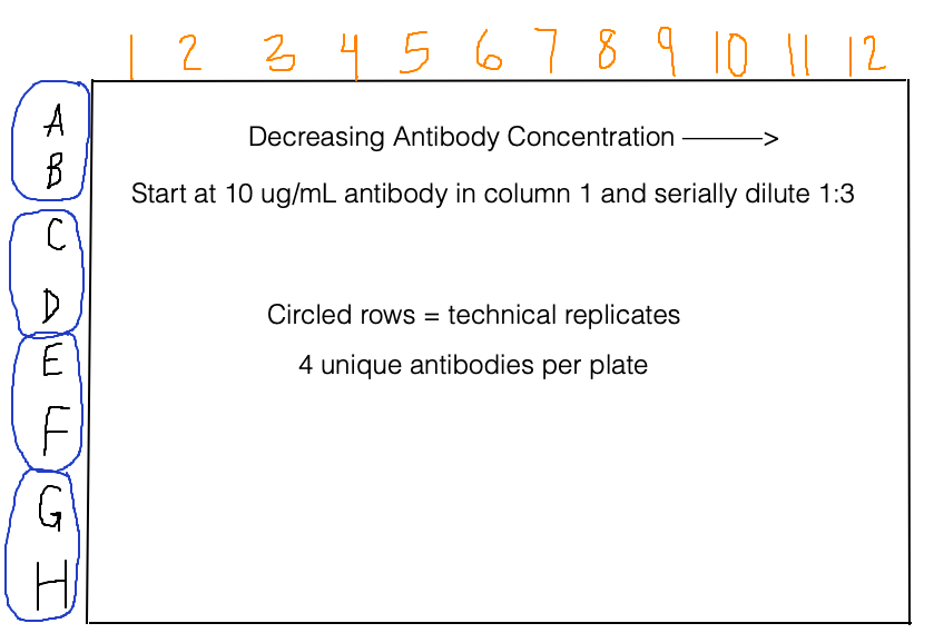
We will first make a list of antibody concentrations, which will be very handy later on. Since the concentrations are serially diluted 1:3 across the plate, we can use an exponential function in a list comprehension to do this:
[3]:
# Units are in ng/mL
ab_concentrations = [10000 * (1 / 3) ** i for i in range(12)]
We will first read in the files, and look at one of them to determine how best to extract the data set. For our purposes, we not keep the metadata, since the main purpose of this exercise is to learn about manipulating data frames. Note that in general you should keep all of the metadata you can.
[4]:
fnames = [f"20200117-{i}.xlsx" for i in range(1, 6)]
df1 = pd.read_excel(os.path.join(data_path, fnames[0]))
# Take a look
df1
[4]:
| Unnamed: 0 | Unnamed: 1 | Unnamed: 2 | Unnamed: 3 | Unnamed: 4 | Unnamed: 5 | Unnamed: 6 | Unnamed: 7 | Unnamed: 8 | Unnamed: 9 | Unnamed: 10 | Unnamed: 11 | Unnamed: 12 | Unnamed: 13 | Unnamed: 14 | |
|---|---|---|---|---|---|---|---|---|---|---|---|---|---|---|---|
| 0 | Software Version | 3.08.01 | NaN | NaN | NaN | NaN | NaN | NaN | NaN | NaN | NaN | NaN | NaN | NaN | NaN |
| 1 | NaN | NaN | NaN | NaN | NaN | NaN | NaN | NaN | NaN | NaN | NaN | NaN | NaN | NaN | NaN |
| 2 | Experiment File Path: | C:\Users\Chou Lab\Desktop\Bjorkman\Andrew\2001... | NaN | NaN | NaN | NaN | NaN | NaN | NaN | NaN | NaN | NaN | NaN | NaN | NaN |
| 3 | Protocol File Path: | NaN | NaN | NaN | NaN | NaN | NaN | NaN | NaN | NaN | NaN | NaN | NaN | NaN | NaN |
| 4 | Plate Number | Plate 1 | NaN | NaN | NaN | NaN | NaN | NaN | NaN | NaN | NaN | NaN | NaN | NaN | NaN |
| 5 | Date | 2020-01-17 00:00:00 | NaN | NaN | NaN | NaN | NaN | NaN | NaN | NaN | NaN | NaN | NaN | NaN | NaN |
| 6 | Time | 15:13:46 | NaN | NaN | NaN | NaN | NaN | NaN | NaN | NaN | NaN | NaN | NaN | NaN | NaN |
| 7 | Reader Type: | Synergy Neo2 | NaN | NaN | NaN | NaN | NaN | NaN | NaN | NaN | NaN | NaN | NaN | NaN | NaN |
| 8 | Reader Serial Number: | 1910162 | NaN | NaN | NaN | NaN | NaN | NaN | NaN | NaN | NaN | NaN | NaN | NaN | NaN |
| 9 | Reading Type | Reader | NaN | NaN | NaN | NaN | NaN | NaN | NaN | NaN | NaN | NaN | NaN | NaN | NaN |
| 10 | NaN | NaN | NaN | NaN | NaN | NaN | NaN | NaN | NaN | NaN | NaN | NaN | NaN | NaN | NaN |
| 11 | Procedure Details | NaN | NaN | NaN | NaN | NaN | NaN | NaN | NaN | NaN | NaN | NaN | NaN | NaN | NaN |
| 12 | Plate Type | 96 WELL PLATE (Use plate lid) | NaN | NaN | NaN | NaN | NaN | NaN | NaN | NaN | NaN | NaN | NaN | NaN | NaN |
| 13 | Eject plate on completion | NaN | NaN | NaN | NaN | NaN | NaN | NaN | NaN | NaN | NaN | NaN | NaN | NaN | NaN |
| 14 | Read | Absorbance Endpoint | NaN | NaN | NaN | NaN | NaN | NaN | NaN | NaN | NaN | NaN | NaN | NaN | NaN |
| 15 | NaN | Full Plate | NaN | NaN | NaN | NaN | NaN | NaN | NaN | NaN | NaN | NaN | NaN | NaN | NaN |
| 16 | NaN | Wavelengths: 450 | NaN | NaN | NaN | NaN | NaN | NaN | NaN | NaN | NaN | NaN | NaN | NaN | NaN |
| 17 | NaN | Read Speed: Normal, Delay: 50 msec, Measurem... | NaN | NaN | NaN | NaN | NaN | NaN | NaN | NaN | NaN | NaN | NaN | NaN | NaN |
| 18 | NaN | NaN | NaN | NaN | NaN | NaN | NaN | NaN | NaN | NaN | NaN | NaN | NaN | NaN | NaN |
| 19 | Results | NaN | NaN | NaN | NaN | NaN | NaN | NaN | NaN | NaN | NaN | NaN | NaN | NaN | NaN |
| 20 | Actual Temperature: | 21 | NaN | NaN | NaN | NaN | NaN | NaN | NaN | NaN | NaN | NaN | NaN | NaN | NaN |
| 21 | NaN | NaN | NaN | NaN | NaN | NaN | NaN | NaN | NaN | NaN | NaN | NaN | NaN | NaN | NaN |
| 22 | NaN | NaN | 1.000 | 2.000 | 3.000 | 4.000 | 5.000 | 6.000 | 7.000 | 8.000 | 9.000 | 10.000 | 11.000 | 12.000 | NaN |
| 23 | NaN | A | 3.104 | 2.900 | 2.849 | 2.756 | 2.402 | 1.721 | 0.954 | 0.452 | 0.190 | 0.096 | 0.063 | 0.055 | 450.0 |
| 24 | NaN | B | 3.022 | 2.610 | 2.565 | 2.740 | 2.238 | 1.622 | 0.946 | 0.422 | 0.186 | 0.092 | 0.066 | 0.054 | 450.0 |
| 25 | NaN | C | 2.894 | 2.786 | 2.702 | 2.544 | 2.252 | 1.570 | 0.864 | 0.374 | 0.165 | 0.091 | 0.063 | 0.054 | 450.0 |
| 26 | NaN | D | 2.724 | 2.749 | 2.776 | 2.595 | 2.153 | 1.576 | 0.861 | 0.376 | 0.167 | 0.088 | 0.063 | 0.053 | 450.0 |
| 27 | NaN | E | 2.634 | 2.653 | 2.596 | 2.449 | 2.139 | 1.447 | 0.755 | 0.330 | 0.168 | 0.083 | 0.077 | 0.053 | 450.0 |
| 28 | NaN | F | 2.735 | 2.747 | 2.726 | 2.546 | 2.155 | 1.435 | 0.772 | 0.336 | 0.151 | 0.086 | 0.062 | 0.059 | 450.0 |
| 29 | NaN | G | 1.178 | 1.103 | 0.817 | 0.579 | 0.319 | 0.154 | 0.079 | 0.068 | 0.056 | 0.061 | 0.051 | 0.049 | 450.0 |
| 30 | NaN | H | 1.305 | 1.061 | 0.884 | 0.549 | 0.299 | 0.165 | 0.084 | 0.061 | 0.053 | 0.056 | 0.050 | 0.051 | 450.0 |
It looks like we can splice out each 96 well plate by keeping only rows 23 to the end and columns 1 to the end. This will work for any excel file taken directly from this particular BioTek plate reader. We will also convert the first column (alphabetic plate rows) to the index column to help with melting the dataframe later on.
[5]:
df1 = pd.read_excel(os.path.join(data_path, fnames[0]), skiprows=22, index_col=1)
# Look at the data frame again
df1.head()
[5]:
| Unnamed: 0 | Unnamed: 2 | Unnamed: 3 | Unnamed: 4 | Unnamed: 5 | Unnamed: 6 | Unnamed: 7 | Unnamed: 8 | Unnamed: 9 | Unnamed: 10 | Unnamed: 11 | Unnamed: 12 | Unnamed: 13 | Unnamed: 14 | |
|---|---|---|---|---|---|---|---|---|---|---|---|---|---|---|
| NaN | NaN | 1.000 | 2.000 | 3.000 | 4.000 | 5.000 | 6.000 | 7.000 | 8.000 | 9.000 | 10.000 | 11.000 | 12.000 | NaN |
| A | NaN | 3.104 | 2.900 | 2.849 | 2.756 | 2.402 | 1.721 | 0.954 | 0.452 | 0.190 | 0.096 | 0.063 | 0.055 | 450.0 |
| B | NaN | 3.022 | 2.610 | 2.565 | 2.740 | 2.238 | 1.622 | 0.946 | 0.422 | 0.186 | 0.092 | 0.066 | 0.054 | 450.0 |
| C | NaN | 2.894 | 2.786 | 2.702 | 2.544 | 2.252 | 1.570 | 0.864 | 0.374 | 0.165 | 0.091 | 0.063 | 0.054 | 450.0 |
| D | NaN | 2.724 | 2.749 | 2.776 | 2.595 | 2.153 | 1.576 | 0.861 | 0.376 | 0.167 | 0.088 | 0.063 | 0.053 | 450.0 |
Reshaping the data set
The first and last columns and the first row can be removed, and we will rename the columns to be the antibody concentrations from our list. We then rename the index and the column header (the name for all of the columns) to useful labels, and we melt!
[6]:
df1 = df1.iloc[1:, 1:-1]
df1.columns = ab_concentrations
df1.index.name = 'Antibody'
df1.columns.name='Ab_Conc_ng_mL'
df1.head()
[6]:
| Ab_Conc_ng_mL | 10000.000000 | 3333.333333 | 1111.111111 | 370.370370 | 123.456790 | 41.152263 | 13.717421 | 4.572474 | 1.524158 | 0.508053 | 0.169351 | 0.056450 |
|---|---|---|---|---|---|---|---|---|---|---|---|---|
| Antibody | ||||||||||||
| A | 3.104 | 2.900 | 2.849 | 2.756 | 2.402 | 1.721 | 0.954 | 0.452 | 0.190 | 0.096 | 0.063 | 0.055 |
| B | 3.022 | 2.610 | 2.565 | 2.740 | 2.238 | 1.622 | 0.946 | 0.422 | 0.186 | 0.092 | 0.066 | 0.054 |
| C | 2.894 | 2.786 | 2.702 | 2.544 | 2.252 | 1.570 | 0.864 | 0.374 | 0.165 | 0.091 | 0.063 | 0.054 |
| D | 2.724 | 2.749 | 2.776 | 2.595 | 2.153 | 1.576 | 0.861 | 0.376 | 0.167 | 0.088 | 0.063 | 0.053 |
| E | 2.634 | 2.653 | 2.596 | 2.449 | 2.139 | 1.447 | 0.755 | 0.330 | 0.168 | 0.083 | 0.077 | 0.053 |
Now we are set to reset the index and melt, preserving the the antibody column as an identifier variable.
[7]:
# Rename columns -- OD450 means optical density at 450 nm
df1 = df1.reset_index().melt(id_vars="Antibody", value_name="OD450")
# Take a look
df1.head()
[7]:
| Antibody | Ab_Conc_ng_mL | OD450 | |
|---|---|---|---|
| 0 | A | 10000.0 | 3.104 |
| 1 | B | 10000.0 | 3.022 |
| 2 | C | 10000.0 | 2.894 |
| 3 | D | 10000.0 | 2.724 |
| 4 | E | 10000.0 | 2.634 |
Putting it all together into a function, we can tidy all three excel files and then concatenate them into a single dataframe.
[8]:
def read_elisa_data(fname):
# Skip the first 22 rows, and make the row names to indices
df = pd.read_excel(fname, skiprows=22, index_col=1)
# Remove the first and last columns and the first row
df = df.iloc[1:, 1:-1]
# Rename the columns to antibody concentrations
df.columns = ab_concentrations
# Assign informative labels
df.index.name = "Antibody"
df.columns.name = "Ab_Conc_ng_mL"
# Melt! Set the new column name as OD450
return df.reset_index().melt(id_vars="Antibody", value_name="OD450")
Each plate has 4 different antibodies, but only one distinct antigen. In this set of experiments, there are two different hepatitis C virus strains and 2 possible mutants (in addition to wild type). The single mutants are called “Q412R” and “Y527H,” which denotes the single amino acid change in them. This information wasn’t stored in the instrument, so it will be manually added to the dataframe. Gotta keep good notes in lab!
I will make a dictionary mapping the plate numbers to the strain names. The plate number (1-5) will be extracted using the rfind method of strings, which returns the index of a particular character. Finally, we use the dictionary to get the strain names and set it to a new column called Antigen. We then separate the Strain and Variant (either wild-type or mutant) by splitting the string at the hyphen.
[9]:
# Dictionary mapping plate number to strain-variant name.
plateIDdict = {
"1": "1a53-Q412R",
"2": "1a157-Q412R",
"3": "1a157-Y527H",
"4": "1a53-WT",
"5": "1a157-WT",
}
df = pd.concat(
[read_elisa_data(os.path.join(data_path, fn)) for fn in fnames],
keys=[plateIDdict[fn[fn.rfind("-") + 1 : fn.rfind(".")]] for fn in fnames],
names=["Antigen"],
).reset_index(level="Antigen")
# Separate the strain and variant from the "Antigen" column
df[["Strain", "Variant"]] = df["Antigen"].str.split("-", expand=True)
# Remove the "Antigen" column
df = df.drop(columns=["Antigen"])
# Take a look at data frame
df.head()
[9]:
| Antibody | Ab_Conc_ng_mL | OD450 | Strain | Variant | |
|---|---|---|---|---|---|
| 0 | A | 10000.0 | 3.104 | 1a53 | Q412R |
| 1 | B | 10000.0 | 3.022 | 1a53 | Q412R |
| 2 | C | 10000.0 | 2.894 | 1a53 | Q412R |
| 3 | D | 10000.0 | 2.724 | 1a53 | Q412R |
| 4 | E | 10000.0 | 2.634 | 1a53 | Q412R |
The very last thing we need to do is rename the rows by antibody. Pairs of adjacent rows are technical replicates, and there are 4 unique antibodies in each plate.
Rows A and B = HEPC74
Rows C and D = HEPC74rua
Rows E and F = HEPC153
Rows G and H = HEPC153rua
There are many ways to do this, but I made a dictionary mapping row letters to antibodies and will use it to replace the values in the row column of the data frame.
[10]:
# Get string of letters (it's not difficult to write out manually,
# but the string package is very useful in more complex cases)
rows = string.ascii_uppercase[:8]
antibodies = ["HEPC74"] * 2 + ["HEPC74rua"] * 2 + ["HEPC153"] * 2 + ["HEPC153rua"] * 2
# Make dictionary
ab_dict = dict(list(zip(rows, antibodies)))
# Replace row names with antibodies
df["Antibody"] = df["Antibody"].map(ab_dict)
# Take a look at data frame
df.head()
[10]:
| Antibody | Ab_Conc_ng_mL | OD450 | Strain | Variant | |
|---|---|---|---|---|---|
| 0 | HEPC74 | 10000.0 | 3.104 | 1a53 | Q412R |
| 1 | HEPC74 | 10000.0 | 3.022 | 1a53 | Q412R |
| 2 | HEPC74rua | 10000.0 | 2.894 | 1a53 | Q412R |
| 3 | HEPC74rua | 10000.0 | 2.724 | 1a53 | Q412R |
| 4 | HEPC153 | 10000.0 | 2.634 | 1a53 | Q412R |
And now we’re done! Everything is tidy, so each absorbance value is associated with a single antigen, antibody, and antibody concentration. Note that the antigen concentrations are all the same (1 μg/mL) in each plate. We can take a look at the mean and standard deviation of the absorbances and verify that they make some sense and we haven’t accidentally reordered things in the data frame—larger antibody concentrations are associated with larger absorbances.
Computing summary statistics
You can also apply methods to groups within a data frame. This is done using pd.groupby.apply. An apply operation can take a long time with larger sets of data and many levels, so you can time how long an apply operation will take using tqdm. The following will be helpful to get going:
import tqdm
tqdm.tqdm.pandas()
pd.groupby([groups]).progress_apply(process_group)
Since we are not using the apply function (I will actually apply a logistic model later in base Python), we won’t go through the details here.
agg() takes a single function (or list of functions) that accept a pd.Series, np.array, list or similar and return a single value summarizing the input. The groupby() agg() combination will do the hard work of aggregating each column of each group with the function/functions passed. Consider calculating the mean and standard deviation of the absorbances).
[11]:
df.groupby(["Strain", "Variant", "Antibody", "Ab_Conc_ng_mL"]).agg([np.mean, np.std])
[11]:
| OD450 | |||||
|---|---|---|---|---|---|
| mean | std | ||||
| Strain | Variant | Antibody | Ab_Conc_ng_mL | ||
| 1a157 | Q412R | HEPC153 | 0.056450 | 0.0600 | 0.005657 |
| 0.169351 | 0.0680 | 0.004243 | |||
| 0.508053 | 0.0735 | 0.007778 | |||
| 1.524158 | 0.1090 | 0.002828 | |||
| 4.572474 | 0.2175 | 0.007778 | |||
| ... | ... | ... | ... | ... | ... |
| 1a53 | WT | HEPC74rua | 123.456790 | 2.3305 | 0.099702 |
| 370.370370 | 2.7750 | 0.022627 | |||
| 1111.111111 | 2.8730 | 0.066468 | |||
| 3333.333333 | 2.7795 | 0.170413 | |||
| 10000.000000 | 2.7730 | 0.261630 | |||
240 rows × 2 columns
Generating plots
In this experiment, we are interested in determining if the different antigen variants bind differently to the same antibody. So we will plot each antibody on a separate plot and color the antigen variants to see the dose-response curve. ELISA data is normally plotted with x axis on a log scale.
[12]:
hv.extension("bokeh")
scatter_plots = hv.Points(
data=df,
kdims=["Ab_Conc_ng_mL", "OD450"], vdims=["Antibody", "Variant", "Strain"],
).groupby(
["Antibody", "Variant", "Strain"]
).opts(
logx=True,
frame_height=200,
frame_width=300,
xlabel="Antibody Concentration (ng/mL)",
size=7,
).overlay(
"Variant"
).layout(
"Strain"
).cols(
1
)
scatter_plots
[12]:
Estimation of the EC50
From ELISA data, we also typically want the half maximal effective concentration, or EC50. It tells you how much antibody concentration you need to reach half of the maximum OD450. This is typically accomplished by obtaining a maximum likelihood estimate (MLE) of parameters of a Hill function,
\begin{align} y = d + \frac{a-d}{1 + \left(\frac{x}{c} \right)^b}. \end{align}
The function has an inverse that can be used to compute the EC50 from the MLE parameters.
\begin{align} x = c \left(\frac{y - a}{d - y}\right)^{1/b} \end{align}
This is a phenomenological approach widely used in the field (but not something Justin recommends). In the functions below, we compute the MLE. We will visit MLE in depth later in the term; for now, take this calculation as a given and as a way to demonstrate application groupby operations.
Importantly, the function compute_ec50() takes as arguments x-values and y-values, performs a MLE, and then returns the resulting EC50.
[13]:
def four_param_hill(x, a, b, c, d):
"""Code up the above 4-parameter Hill function"""
return d + (a - d) / (1 + (x / c) ** b)
def inverse_four_param_hill(y, a, b, c, d):
"""Inverse of the four parameter fit in order to compute concentration from absorbance"""
return c * ((y - a) / (d - y)) ** (1 / b)
def compute_ec50(x, y):
# Perform the fit using scipy and save the optimal parameters (popt)
popt, _ = scipy.optimize.curve_fit(four_param_hill, x, y)
# Compute the expected values from the logistic regression
fit = np.array(four_param_hill(x, *popt))
# Compute the half maximal value in order to find the EC50
halfway = (np.min(fit) + np.max(fit)) / 2
ec50 = inverse_four_param_hill(halfway, *popt)
return ec50
We wish to compute the EC50 for each strain/variant/antibody combination. To do so, we group by through three variables and apply the compute_ec50() function. Any function we wish to apply needs to take a group (a sub-data frame) as an argument. So, we can write a lambda function to call compute_fit().
[14]:
ec50_results = df.groupby(["Strain", "Variant", "Antibody"]).apply(
lambda group: compute_ec50(group["Ab_Conc_ng_mL"].values, group["OD450"].values)
)
# Take a look
ec50_results
[14]:
Strain Variant Antibody
1a157 Q412R HEPC153 80.001005
HEPC153rua 1191.675379
HEPC74 37.760901
HEPC74rua 63.641514
WT HEPC153 40.358598
HEPC153rua 3353.090522
HEPC74 26.682279
HEPC74rua 33.763761
Y527H HEPC153 34.673164
HEPC153rua 391.143463
HEPC74 24.829800
HEPC74rua 27.293204
1a53 Q412R HEPC153 36.874215
HEPC153rua 509.791761
HEPC74 30.436993
HEPC74rua 33.391581
WT HEPC153 36.111559
HEPC153rua 599.556461
HEPC74 27.502283
HEPC74rua 31.517035
dtype: float64
The result is a Pandas series with a multiindex. We can convert this to a data frame by resetting the index, and then sort by strain and antibody for convenience.
[15]:
# Set the name of the series
ec50_results.name = "EC50"
# Convert to data frame and sort
ec50_results.reset_index().sort_values(by=["Strain", "Antibody"]).reset_index(drop=True)
[15]:
| Strain | Variant | Antibody | EC50 | |
|---|---|---|---|---|
| 0 | 1a157 | Q412R | HEPC153 | 80.001005 |
| 1 | 1a157 | WT | HEPC153 | 40.358598 |
| 2 | 1a157 | Y527H | HEPC153 | 34.673164 |
| 3 | 1a157 | Q412R | HEPC153rua | 1191.675379 |
| 4 | 1a157 | WT | HEPC153rua | 3353.090522 |
| 5 | 1a157 | Y527H | HEPC153rua | 391.143463 |
| 6 | 1a157 | Q412R | HEPC74 | 37.760901 |
| 7 | 1a157 | WT | HEPC74 | 26.682279 |
| 8 | 1a157 | Y527H | HEPC74 | 24.829800 |
| 9 | 1a157 | Q412R | HEPC74rua | 63.641514 |
| 10 | 1a157 | WT | HEPC74rua | 33.763761 |
| 11 | 1a157 | Y527H | HEPC74rua | 27.293204 |
| 12 | 1a53 | Q412R | HEPC153 | 36.874215 |
| 13 | 1a53 | WT | HEPC153 | 36.111559 |
| 14 | 1a53 | Q412R | HEPC153rua | 509.791761 |
| 15 | 1a53 | WT | HEPC153rua | 599.556461 |
| 16 | 1a53 | Q412R | HEPC74 | 30.436993 |
| 17 | 1a53 | WT | HEPC74 | 27.502283 |
| 18 | 1a53 | Q412R | HEPC74rua | 33.391581 |
| 19 | 1a53 | WT | HEPC74rua | 31.517035 |
We’ve almost completely recreated the ELISA plotting in Prism, a common subscription software used by biologists to plot all sorts of data. We also didn’t have to copy and paste columns and rows from Excel over and over again.
In EC50 values, we are interested in the smaller numbers because they indicate that LESS antibody was required to achieve the same signal. It appears that our mutants have a mix of larger and smaller EC50 values relative to the wild-type strains.
We could also plot the regression lines on the same plots with the points to do a visual test of the EC50 estimates. We do not do this here, opting instead to wait for the discussion on MLE and visualization of the results later in the course.
Computing Environment
[16]:
%load_ext watermark
%watermark -v -p numpy,scipy,pandas,bokeh,holoviews,bebi103,jupyterlab
Python implementation: CPython
Python version : 3.8.12
IPython version : 7.27.0
numpy : 1.21.2
scipy : 1.7.1
pandas : 1.3.3
bokeh : 2.3.3
holoviews : 1.14.6
bebi103 : 0.1.8
jupyterlab: 3.1.7