21. Implementation of hierarchical models
[1]:
# Colab setup ------------------
import os, sys, subprocess
if "google.colab" in sys.modules:
cmd = "pip install --upgrade colorcet bebi103 arviz cmdstanpy watermark"
process = subprocess.Popen(cmd.split(), stdout=subprocess.PIPE, stderr=subprocess.PIPE)
stdout, stderr = process.communicate()
import cmdstanpy; cmdstanpy.install_cmdstan()
data_path = "https://s3.amazonaws.com/bebi103.caltech.edu/data/"
else:
data_path = "../data/"
# ------------------------------
import io
import numpy as np
import pandas as pd
import cmdstanpy
import arviz as az
import bebi103
import iqplot
import bokeh.io
bokeh.io.output_notebook()


In the previous lesson, we learned about how to construct hierarchical models and how to sample from the resulting posterior distribution. In this lesson, we will dig a bit deeper and address some of the challenges in sampling out of hierarchical models.
Hierarchical model structure
To think about the structure of hierarchical models, we will consider the following experimental design. We are measuring fluorescent intensity of a reporter of gene expression in E. coli cells. One Monday, we prepare four batches of E. coli and grow them up on plates. From each plate, we select colonies. We then mount a slide with a selection from a given colony and use fluorescence microscopy to determine the fluorescence level of individual cells. We do a similar experiment on Wednesday, and then another on Thursday. We model the measured fluorescence values as Normally distributed.
There is a hierarchical structure here, depicted below.
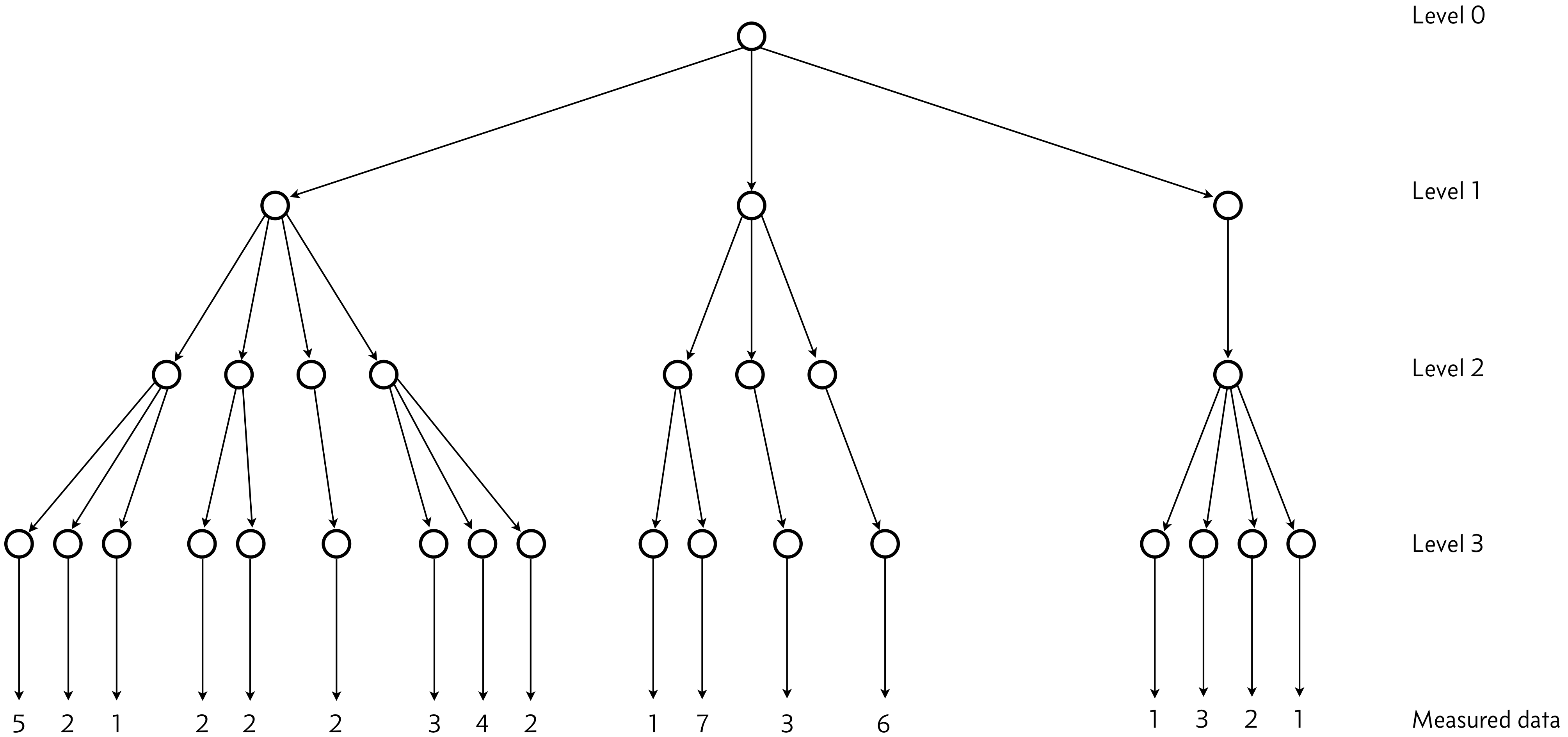
Level 0: This level has the hyperparameters \(\theta\) and \(\sigma\), the location and scale parameters of fluorescence intensity typical of an E. coli cell expressing the fluorescent gene of interest. These are the parameters we ultimately wish to get estimates for.
Level 1 corresponds to the day the experiment was performed. There will be variability from day to day, and the location and scale parameters for a given day are conditioned on the hyperparameters, but can vary from the parameters of other days.
Level 2 corresponds to which batch of cells were used on a given day.
Level 3 corresponds to the colony of cells chosen from the batch.
The colony-level information then informs the data. In the above diagram, I have indicated how many individual cells are measured in each microscope experiment.
The structure here shows the conditioning. The measured data are parametrized by the colony-level information, which is itself parametrized by the batch-level information, which is itself parametrized by the day-level information, which is finally parametrized by the hyperparameters at the root of the hierarchy.
To keep track of all the hyperparameters, it is easiest to define arrays for the hyperparameters at each level. In this example, we have
\begin{align} &\text{Level 0 parameter: }\phantom{\text{s}} \theta \\[1em] &\text{Level 1 parameters: } \theta_1 \equiv (\theta_1^1, \theta_1^2, \theta_1^3) \\[1em] &\text{Level 2 parameters: } \theta_2 \equiv (\theta_2^1, \theta_2^2, \theta_2^3, \ldots \theta_2^8) \\[1em] &\text{Level 3 parameters: } \theta_3 \equiv (\theta_3^1, \theta_3^2, \theta_3^3, \ldots \theta_3^{17}). \end{align}
To complete the formalization of the specification, we need arrays that tell us which upon which hyperparameter each parameter is conditioned. Level 1 is special because it is conditioned only by \(\theta\). The respective elements in the level 2 parameters are conditioned by the following level 1 conditioners.
\begin{align} &\text{level 1 hyperparameter conditioners: } (\theta_1^1, \theta_1^1, \theta_1^1, \theta_1^1, \theta_1^2, \theta_1^2, \theta_1^2, \theta_1^3). \end{align}
To avoid all of the subscripting and superscripting, we can write this as
\begin{align} \text{index 1: } (1, 1, 1, 1, 2, 2, 2, 3), \end{align}
with level 3’s conditioners in level 2 being
\begin{align} \text{index 2: } (1, 1, 1, 2, 2, 3, 4, 4, 4, 5, 5, 6, 7, 8, 8, 8, 8), \end{align}
and finally the data conditioned by level 3’s parameters,
\begin{align} \text{index 3: } (&1, 1, 1, 1, 1, 2, 2, 3, 4, 4, 5, 5, 6, 6, 7, 7, 7,\\ &8, 8, 8, 8, 9, 9, 10, 11, 11, 11, 11, 11, 11, 11, 12, 12, 12,\\ &13, 13, 13, 13, 13, 13, 14, 15, 15, 15, 16, 16, 17). \end{align}
We define that there are \(J_1\) parameters in level 1, \(J_2\) in level 2, and generically \(J_k\) in level \(k\). In this case,
\begin{align} &J_1 = 3,\\[1em] &J_2 = 8,\\[1em] &J_3 = 17.\\[1em] \end{align}
To have a concrete model in mind, we will assume that all colonies have the same scale parameter, but differing location parameters. We assume further that all hyperparameters are dependent on those at a level above by a Normal relationship, and we assume the same variance \(\tau\) for relationships all the way down the hierarchy. That is \(\tau\) applies for conditioning level 3 on level 2, level 2 on level 1, and level 1 on level 0. We consider a hyperprior for \(\theta\) to be a Normal distribution centered on 10 arbitrary fluorescence units with a standard deviation of 3, and \(\sigma\) to have a Half-Normal prior. Our statistical model is then defined as follows, with a weakly informative hyperprior on \(\tau\).
\begin{align} &\theta \sim \text{Norm}(10, 3) \\[1em] &\tau \sim \text{HalfNorm}(5) \\[1em] &\theta_1 \sim \text{Norm}(\theta, \tau) \\[1em] &\theta_2 \sim \text{Norm}(\theta_1, \tau) \\[1em] &\theta_3 \sim \text{Norm}(\theta_2, \tau) \\[1em] &\sigma \sim \text{HalfNorm}(5) \\[1em] &y \sim \text{Norm}(\theta_3, \sigma). \end{align}
Here, we have defined the measurements as \(y\), and we have implied that the appropriate conditioning on which specific hyperparameters (as given by index 1, index 2, and index 3 defined above) is considered.
This method of organization is useful to keep conditioning straight in hierarchical models. As we will see momentarily, it is also convenient for implementing a hierarchical model in Stan.
Coding up the hierarchical model in Stan
Provided we can define arrays for index 1, index 2, and index 3, coding the model up in Stan is surprisingly straightforward. To start, we will use a centered parametrization for clarity. (We will see the problems this causes with sampling momentarily.) Here is a Stan code for the hierarchical model.
data {
// Total number of data points
int N;
// Number of entries in each level of the hierarchy
int J_1;
int J_2;
int J_3;
//Index arrays to keep track of hierarchical structure
int index_1[J_2];
int index_2[J_3];
int index_3[N];
// The measurements
real y[N];
}
parameters {
// Hyperparameters level 0
real theta;
// How hyperparameters vary
real<lower=0> tau;
// Hyperparameters level 1
vector[J_1] theta_1;
// Hyperparameters level 2
vector[J_2] theta_2;
// Parameters
vector[J_3] theta_3;
real<lower=0> sigma;
}
model {
theta ~ normal(10, 3);
tau ~ normal(0, 5);
theta_1 ~ normal(theta, tau);
theta_2 ~ normal(theta_1[index_1], tau);
theta_3 ~ normal(theta_2[index_2], tau);
sigma ~ normal(0, 5);
y ~ normal(theta_3[index_3], sigma);
}
Be sure to carefully read the Stan code. Importantly, note that theta_1,theta_2, and theta_3 are vector valued. Note also that we use indexing to specify which parameters correspond to which day, batch, and colony. In studying the code and the model above, you should be able to see how the hierarchical model is built in Stan.
A quick aside: generating a data set
I will now generate a tidy data frame containing a data set to analyze with this hierarchical model. These are fabricated data, hence the weird loading with a string (for compactness so we don’t have a big code cell).
[2]:
data_str = "".join(
[
"day,batch,colony,y\nm,1,1,11.40\nm,1,1,10.54\n",
"m,1,1,12.17\nm,1,1,12.41\nm,1,1,9.97\nm,1,2,10.76\n",
"m,1,2,9.16\nm,1,3,9.50\nm,2,1,9.34\nm,2,1,10.14\n",
"m,2,2,10.72\nm,2,2,10.63\nm,3,1,11.37\nm,3,1,10.51\n",
"m,4,1,11.06\nm,4,1,10.68\nm,4,1,12.58\nm,4,2,11.21\n",
"m,4,2,11.07\nm,4,2,10.74\nm,4,2,11.68\nm,4,3,10.65\n",
"m,4,3,9.06\nw,1,1,10.40\nw,1,2,10.75\nw,1,2,11.42\n",
"w,1,2,10.42\nw,1,2,9.18\nw,1,2,10.69\nw,1,2,9.37\n",
"w,1,2,11.32\nw,2,1,9.90\nw,2,1,10.53\nw,2,1,10.76\n",
"w,3,1,11.08\nw,3,1,9.27\nw,3,1,12.01\nw,3,1,12.20\n",
"w,3,1,11.23\nw,3,1,10.96\nr,1,1,9.73\nr,1,2,11.25\n",
"r,1,2,9.99\nr,1,2,10.12\nr,1,3,9.65\nr,1,3,10.18\nr,1,4,12.70\n",
]
)
data_str = (
data_str.replace("m", "monday").replace("w", "wednesday").replace("r", "thursday")
)
df = pd.read_csv(io.StringIO(data_str))
# Take a look
df.head()
[2]:
| day | batch | colony | y | |
|---|---|---|---|---|
| 0 | monday | 1 | 1 | 11.40 |
| 1 | monday | 1 | 1 | 10.54 |
| 2 | monday | 1 | 1 | 12.17 |
| 3 | monday | 1 | 1 | 12.41 |
| 4 | monday | 1 | 1 | 9.97 |
The data are tidy with each row corresponding to a measurement with the appropriate metadata present to determine which day, batch, and colony the measurement was from. Let’s take a quick graphical look at the data set. We will color each data point by the colony number and group by day and batch.
[3]:
bokeh.io.show(
iqplot.strip(
df,
q="y",
cats=["day", "batch"],
color_column="colony",
marker_kwargs=dict(alpha=0.6),
)
)
Generating input data for Stan
We should now convert the data frame into a data dictionary that Stan likes, adhering to our more general hierarchical model specification above, i.e., replacing 'day' with 'index_1', 'batch' with 'index_2' and 'colony' with 'index_3'. Importantly, we should update the original data frame to include these indices (which will be included in Stan’s output) that match the respective categorical parameters in the original data set. The function
bebi103.stan.df_to_datadict_hier() does this. You need to specify the tidy data frame you want to convey, the columns of the data frame corresponding to the levels of the hierarchy in order of the hierarchy, and the column(s) that have the measured data.
[4]:
data, df = bebi103.stan.df_to_datadict_hier(
df, level_cols=["day", "batch", "colony"], data_cols="y"
)
# Take a look at the data dictionary
data
[4]:
{'N': 47,
'J_1': 3,
'J_2': 8,
'J_3': 17,
'index_1': array([1, 1, 1, 1, 2, 3, 3, 3]),
'index_2': array([1, 1, 1, 2, 2, 3, 4, 4, 4, 5, 5, 5, 5, 6, 6, 7, 8]),
'index_3': array([ 1, 1, 1, 1, 1, 2, 2, 3, 4, 4, 5, 5, 6, 6, 7, 7, 7,
8, 8, 8, 8, 9, 9, 10, 11, 11, 11, 12, 12, 13, 14, 15, 15, 15,
15, 15, 15, 15, 16, 16, 16, 17, 17, 17, 17, 17, 17]),
'y': array([11.4 , 10.54, 12.17, 12.41, 9.97, 10.76, 9.16, 9.5 , 9.34,
10.14, 10.72, 10.63, 11.37, 10.51, 11.06, 10.68, 12.58, 11.21,
11.07, 10.74, 11.68, 10.65, 9.06, 9.73, 11.25, 9.99, 10.12,
9.65, 10.18, 12.7 , 10.4 , 10.75, 11.42, 10.42, 9.18, 10.69,
9.37, 11.32, 9.9 , 10.53, 10.76, 11.08, 9.27, 12.01, 12.2 ,
11.23, 10.96])}
It is also instructive to look at the entire updated data frame so you can understand how the labeling of indices works.
[5]:
df
[5]:
| day | batch | colony | y | day_stan | batch_stan | colony_stan | |
|---|---|---|---|---|---|---|---|
| 0 | monday | 1 | 1 | 11.40 | 1 | 1 | 1 |
| 1 | monday | 1 | 1 | 10.54 | 1 | 1 | 1 |
| 2 | monday | 1 | 1 | 12.17 | 1 | 1 | 1 |
| 3 | monday | 1 | 1 | 12.41 | 1 | 1 | 1 |
| 4 | monday | 1 | 1 | 9.97 | 1 | 1 | 1 |
| 5 | monday | 1 | 2 | 10.76 | 1 | 1 | 2 |
| 6 | monday | 1 | 2 | 9.16 | 1 | 1 | 2 |
| 7 | monday | 1 | 3 | 9.50 | 1 | 1 | 3 |
| 8 | monday | 2 | 1 | 9.34 | 1 | 2 | 4 |
| 9 | monday | 2 | 1 | 10.14 | 1 | 2 | 4 |
| 10 | monday | 2 | 2 | 10.72 | 1 | 2 | 5 |
| 11 | monday | 2 | 2 | 10.63 | 1 | 2 | 5 |
| 12 | monday | 3 | 1 | 11.37 | 1 | 3 | 6 |
| 13 | monday | 3 | 1 | 10.51 | 1 | 3 | 6 |
| 14 | monday | 4 | 1 | 11.06 | 1 | 4 | 7 |
| 15 | monday | 4 | 1 | 10.68 | 1 | 4 | 7 |
| 16 | monday | 4 | 1 | 12.58 | 1 | 4 | 7 |
| 17 | monday | 4 | 2 | 11.21 | 1 | 4 | 8 |
| 18 | monday | 4 | 2 | 11.07 | 1 | 4 | 8 |
| 19 | monday | 4 | 2 | 10.74 | 1 | 4 | 8 |
| 20 | monday | 4 | 2 | 11.68 | 1 | 4 | 8 |
| 21 | monday | 4 | 3 | 10.65 | 1 | 4 | 9 |
| 22 | monday | 4 | 3 | 9.06 | 1 | 4 | 9 |
| 40 | thursday | 1 | 1 | 9.73 | 2 | 5 | 10 |
| 41 | thursday | 1 | 2 | 11.25 | 2 | 5 | 11 |
| 42 | thursday | 1 | 2 | 9.99 | 2 | 5 | 11 |
| 43 | thursday | 1 | 2 | 10.12 | 2 | 5 | 11 |
| 44 | thursday | 1 | 3 | 9.65 | 2 | 5 | 12 |
| 45 | thursday | 1 | 3 | 10.18 | 2 | 5 | 12 |
| 46 | thursday | 1 | 4 | 12.70 | 2 | 5 | 13 |
| 23 | wednesday | 1 | 1 | 10.40 | 3 | 6 | 14 |
| 24 | wednesday | 1 | 2 | 10.75 | 3 | 6 | 15 |
| 25 | wednesday | 1 | 2 | 11.42 | 3 | 6 | 15 |
| 26 | wednesday | 1 | 2 | 10.42 | 3 | 6 | 15 |
| 27 | wednesday | 1 | 2 | 9.18 | 3 | 6 | 15 |
| 28 | wednesday | 1 | 2 | 10.69 | 3 | 6 | 15 |
| 29 | wednesday | 1 | 2 | 9.37 | 3 | 6 | 15 |
| 30 | wednesday | 1 | 2 | 11.32 | 3 | 6 | 15 |
| 31 | wednesday | 2 | 1 | 9.90 | 3 | 7 | 16 |
| 32 | wednesday | 2 | 1 | 10.53 | 3 | 7 | 16 |
| 33 | wednesday | 2 | 1 | 10.76 | 3 | 7 | 16 |
| 34 | wednesday | 3 | 1 | 11.08 | 3 | 8 | 17 |
| 35 | wednesday | 3 | 1 | 9.27 | 3 | 8 | 17 |
| 36 | wednesday | 3 | 1 | 12.01 | 3 | 8 | 17 |
| 37 | wednesday | 3 | 1 | 12.20 | 3 | 8 | 17 |
| 38 | wednesday | 3 | 1 | 11.23 | 3 | 8 | 17 |
| 39 | wednesday | 3 | 1 | 10.96 | 3 | 8 | 17 |
We now have the necessary data for Stan’s sampler.
Drawing samples and checking diagnostics
So, let’s sample and see what we get!
[6]:
with bebi103.stan.disable_logging():
sm_centered = cmdstanpy.CmdStanModel(stan_file='centered.stan')
samples_centered = sm_centered.sample(data=data, seed=3252)
samples_centered = az.from_cmdstanpy(posterior=samples_centered)
That was fast! Hopefully everything worked ok for this model. Let’s start by checking all of the dianostics to see if there were any issues.
[7]:
bebi103.stan.check_all_diagnostics(samples_centered)
ESS for parameter tau is 81.75398022675449.
tail-ESS for parameter tau is 88.58505421313811.
tail-ESS for parameter theta_1[0] is 336.0488203003088.
tail-ESS for parameter theta_2[1] is 358.8781526234507.
ESS for parameter theta_3[3] is 309.3988332722338.
tail-ESS for parameter theta_3[3] is 260.3296226542579.
ESS for parameter theta_3[11] is 359.6351942098255.
ESS or tail-ESS below 100 per chain indicates that expectation values
computed from samples are unlikely to be good approximations of the
true expectation values.
Rhat for parameter theta is 1.0128984905475433.
Rhat for parameter tau is 1.067936523093342.
Rhat for parameter theta_1[0] is 1.0122136667824546.
Rhat for parameter theta_2[0] is 1.0133051913295972.
Rhat for parameter theta_2[1] is 1.01283859015507.
Rhat for parameter theta_2[5] is 1.0142534269819143.
Rhat for parameter theta_2[6] is 1.0138172354210306.
Rhat for parameter theta_3[1] is 1.0115813151712891.
Rhat for parameter theta_3[2] is 1.0105468486798657.
Rhat for parameter theta_3[6] is 1.0100074876844278.
Rhat for parameter theta_3[8] is 1.0113563141021014.
Rhat for parameter theta_3[9] is 1.0134524978790296.
Rhat for parameter theta_3[11] is 1.011537889456516.
Rhat for parameter theta_3[12] is 1.0211605322078865.
Rhat for parameter theta_3[13] is 1.0112481744615087.
Rhat for parameter theta_3[14] is 1.012537612648559.
Rhat for parameter theta_3[15] is 1.0100218681126796.
Rank-normalized Rhat above 1.01 indicates that the chains very likely have not mixed.
7 of 4000 (0.175%) iterations ended with a divergence.
Try running with larger adapt_delta to remove divergences.
0 of 4000 (0.0%) iterations saturated the maximum tree depth of 10.
Chain 0: E-BFMI = 0.055957419005010285
Chain 1: E-BFMI = 0.1093611678874502
Chain 2: E-BFMI = 0.07787734789756103
Chain 3: E-BFMI = 0.07468263585646949
E-BFMI below 0.3 indicates you may need to reparametrize your model.
[7]:
23
Whew! Lots of problems here. Most strikingly, the effective sample size for \(\tau\) is very small. Furthermore, there are a few divergences. Not many, and they could be false positives, but we should check to see if there is a pattern to the divergences. To start looking for the pattern, let’s make a parallel coordinate plot.
[8]:
parameters = (
["theta", "sigma", "tau"]
+ [f"theta_1[{i}]" for i in samples_centered.posterior.theta_1_dim_0.values]
+ [f"theta_2[{i}]" for i in samples_centered.posterior.theta_2_dim_0.values]
+ [f"theta_3[{i}]" for i in samples_centered.posterior.theta_3_dim_0.values]
)
bokeh.io.show(
bebi103.viz.parcoord(
samples_centered,
parameters=parameters,
xtick_label_orientation="vertical",
transformation="minmax",
)
)
Even though there are very few divergences, they all go through low \(\tau\). This is a symptom of hitting a funnel. We can see this in the corner plot.
[9]:
bokeh.io.show(
bebi103.viz.corner(samples_centered, parameters=["theta", "sigma", "tau"])
)
Looking at the tau versus theta plot, we see that the divergences are for small tau. Zooming in on the bottom of that plot shows that the sampler is hitting the entry to a funnel; it cannot sample down to tau values close to zero. We can possibly alleviate this problem by uncentering the model.
A noncentered parametrization
To uncenter the model, we reparametrize our model as follows.
\begin{align} &\theta \sim \text{Norm}(10, 3) \\[1em] &\tau \sim \text{HalfNorm}(5) \\[1em] &\tilde{\theta}_1 \sim \text{Norm}(0, 1) \\[1em] &\theta_1 = \theta + \tau \tilde{\theta}_1 \\[1em] &\tilde{\theta}_2 \sim \text{Norm}(0, 1) \\[1em] &\theta_2 = \theta_1 + \tau \tilde{\theta}_2 \\[1em] &\tilde{\theta}_3 \sim \text{Norm}(0, 1) \\[1em] &\theta_3 = \theta_2 + \tau \tilde{\theta}_3 \\[1em] &\sigma \sim \text{HalfNorm}(5) \\[1em] &y \sim \text{Norm}(\theta_3, \sigma). \end{align}
This frees the sampler to explore standard Normal distributions and then uses a transformation to sample the funnel. The models is called “noncentered” because the sampling is done around a value of zero, not the center of the \(\theta\) distributions. We can then recenter these noncentered samples by applying a transformation such as \(\theta_1 = \theta + \tau \tilde{\theta}_1\), where \(\tilde{\theta}_1\) are the noncentered samples.
Let’s code this up in Stan. The Stan code is:
data {
// Total number of data points
int N;
// Number of entries in each level of the hierarchy
int J_1;
int J_2;
int J_3;
//Index arrays to keep track of hierarchical structure
int index_1[J_2];
int index_2[J_3];
int index_3[N];
// The measurements
real y[N];
}
parameters {
// Hyperparameters level 0
real theta;
// How hyperparameters vary
real<lower=0> tau;
// Hyperparameters level 1
vector[J_1] theta_1_tilde;
// Hyperparameters level 2
vector[J_2] theta_2_tilde;
// Parameters
vector[J_3] theta_3_tilde;
real<lower=0> sigma;
}
transformed parameters {
// Transformations from noncentered
vector[J_1] theta_1 = theta + tau * theta_1_tilde;
vector[J_2] theta_2 = theta_1[index_1] + tau * theta_2_tilde;
vector[J_3] theta_3 = theta_2[index_2] + tau * theta_3_tilde;
}
model {
theta ~ normal(10, 3);
tau ~ normal(0, 5);
theta_1_tilde ~ normal(0, 1);
theta_2_tilde ~ normal(0, 1);
theta_3_tilde ~ normal(0, 1);
sigma ~ normal(0, 5);
y ~ normal(theta_3[index_3], sigma);
}
Let’s draw our samples and see if we were able to alleviate the problems we diagnosed with the centered parametrizations.
[10]:
with bebi103.stan.disable_logging():
sm_noncentered = cmdstanpy.CmdStanModel(stan_file='noncentered.stan')
samples_noncentered = sm_noncentered.sample(data=data, seed=3252)
samples_noncentered = az.from_cmdstanpy(posterior=samples_noncentered)
Let’s first check the diagnostics.
[11]:
bebi103.stan.check_all_diagnostics(samples_noncentered)
Effective sample size looks reasonable for all parameters.
Rhat looks reasonable for all parameters.
3 of 4000 (0.075%) iterations ended with a divergence.
Try running with larger adapt_delta to remove divergences.
0 of 4000 (0.0%) iterations saturated the maximum tree depth of 10.
E-BFMI indicated no pathological behavior.
[11]:
4
The problems with effective sample size and Rhat are gone, but we still have divergences. Let’s again take a look at where the divergences are coming from with a parallel coordinate plot.
[12]:
bokeh.io.show(
bebi103.viz.parcoord(
samples_noncentered,
parameters=parameters,
xtick_label_orientation="vertical",
transformation="minmax",
)
)
It is hard to see an immediate pattern in the divergences here. Let’s look at the corner plot to see if anything is obvious.
[13]:
bokeh.io.show(
bebi103.viz.corner(samples_noncentered, parameters=["theta", "sigma", "tau"])
)
There does not seem to be any apparent pattern in the divergences, which means that they could be false positives. We can deal with them by increasing the adapt_delta parameter of the sampler, which I won’t do here (you can try it yourself; it works). Importantly, zooming in on the tau versus theta plot shows that the sampler is now properly sampling small values of \(\tau\), effectively sampling down toward zero. We can see this more clearly by comparing the samples from the
centered versus noncentered parametrizations with \(\tau\) on a logarithmic scale.
[14]:
p = bokeh.plotting.figure(
height=400, width=450, x_axis_label="θ", y_axis_label="τ", y_axis_type="log"
)
p.circle(
samples_centered.posterior.theta.values.flatten(),
samples_centered.posterior.tau.values.flatten(),
legend_label="centered",
alpha=0.2,
)
p.circle(
samples_noncentered.posterior.theta.values.flatten(),
samples_noncentered.posterior.tau.values.flatten(),
legend_label="noncentered",
color="orange",
alpha=0.2,
)
p.legend.location = "bottom_right"
p.legend.click_policy = "hide"
bokeh.io.show(p)
We have much better sampling for low \(\tau\). Let’s think for a moment about why this is important. A large value of \(\tau\) means that the parameters governing the outcomes of the respective experiments are essentially independent. A small value of \(\tau\) means that the parameters governing the experiments are all nearly the same. Thus, small \(\tau\) corresponds to pooling all of the results together in a single data set. So, you can think of \(\tau\) like a slider; small \(\tau\) gives the extreme model where the experiments are all pooled together, and large \(\tau\) gives the opposite extreme, where the experiments are all independent. The whole point of using a hierarchical model is to capture all of the possible behavior between (and including) these two extremes. If we cannot effectively sample \(\tau\), we are not capturing the possible structure of the data set.
Conclusions
Hierarchical modeling presents special challenges for samplers. There are tricks we can do to improve the performance of HMC samplers in exploring the parameter space, such as using noncentered parametrizations and encouraging the sampler to take smaller steps by tuning the adapt_delta parameter. Importantly, though, you should carefully check the diagnostics of your sampler. This is true even if you are not working with a hierarchical model.
[15]:
bebi103.stan.clean_cmdstan()
[16]:
%load_ext watermark
%watermark -v -p numpy,pandas,cmdstanpy,arviz,bokeh,iqplot,bebi103,jupyterlab
print("cmdstan :", bebi103.stan.cmdstan_version())
Python implementation: CPython
Python version : 3.8.5
IPython version : 7.19.0
numpy : 1.19.2
pandas : 1.2.1
cmdstanpy : 0.9.67
arviz : 0.11.0
bokeh : 2.2.3
iqplot : 0.2.0
bebi103 : 0.1.2
jupyterlab: 2.2.6
cmdstan : 2.26.0