R3. Choosing priors

This recitation was conducted by Cece Andrews and Ariana Tribby.

---

# Colab setup ------------------
import os, sys, subprocess
if "google.colab" in sys.modules:
    cmd = "pip install --upgrade iqplot watermark"
    process = subprocess.Popen(cmd.split(), stdout=subprocess.PIPE, stderr=subprocess.PIPE)
    stdout, stderr = process.communicate()
    data_path = "https://s3.amazonaws.com/bebi103.caltech.edu/data/"
else:
    data_path = "../data/"
# ------------------------------

import numpy as np
import pandas as pd

import iqplot

import bokeh.io
bokeh.io.output_notebook()

import scipy.special
import scipy.optimize
import scipy.stats as st

Loading BokehJS ...

---

Part 1: Review of Lecture

In Part 1 we reviewed the Lecture 2 section on choosing priors. A quick recap of what we learned:

1. Uniform prior: Not the best. Improper prior – it gives us no information and is not normalizable!

2. Jeffreys prior: Also not great. Fixes the problem of the uniform prior where the priors vary with change of variables, but it is very hard to compute for some distributions.

3. Weakly informative prior: Good! We can choose a prior probability distribution to encode what we know about the parameter before we measured data. We will discuss how to come up with weakly informative priors below.

4. Conjugate prior: Can be helpful! Makes the posterior possible to analyze analytically, but only a few distributions have conjugates, so not always possible.

Part 2: Tips and Practice for Choosing Weakly Informative Priors

Recommended steps for choosing priors:

1. Write down Bayes’ Theorem first!

\begin{align} g(\mu \mid y) = \frac{f(y\mid \mu )\,g(\mu )}{f(y)}. \end{align}

In words: \begin{align} \text{posterior} = \frac{\text{likelihood}\,x\ \text{prior}}{\text{evidence}} \end{align}

2. Choose your likelihood (please see Recitation 2/Lecture 2 for help).

3. Assuming the parameters are independently distributed in the prior, you will need to choose a prior for each parameter in your likelihood. For example, if you choose \(f(y\mid \mu )\sim\text{Normal}(\mu, \sigma)\), you will need to choose priors \(g(\mu)\) and \(g(\sigma)\).

4. Consider what you know about the parameter. Do you know what it means in the system? Are there any bounds on its value? Is it related to other parameters? Will its value be very close to zero/very far from zero?

5. Come up with a sketch of what you think the probability distribution for your prior will look like. Your sketch should cover all possible values of the parameter.

6. Use the Distribution Explorer to help you choose a probability distribution that matches your sketch. Consider the story and shape of the distribution. Play around with the distribution explorer, how does changing the parameters change the shape of the distribution?

7. Go for more broad instead of more narrow!

8. Don’t stress too much! Most often there will be several reasonable choices for priors. And they will be overwhelmed by the likelihood. As long as your prior is reasonable and not overly narrow, you will be fine!

We will now do a couple examples of choosing priors with data used in previous terms/years of the course. In these examples we will not worry too much about the likelihood and focus more on practicing choosing priors.

Example 1: Spindle Size

From our favorite data set involving mitotic spindle sizes….

“The data set we will use for this analysis comes from Good, et al., Cytoplasmic volume modulates spindle size during embryogenesis Science, 342, 856-860, 2013. You can download the data set here. In this work, Matt Good and coworkers developed a microfluidic device where they could create droplets cytoplasm extracted from Xenopus eggs and embryos (see figure below; scale bar 20 µm). A remarkable property about Xenopus extract is that mitotic spindles spontaneously form; the extracted cytoplasm has all the ingredients to form them. This makes it an excellent model system for studying spindles. With their device, Good and his colleagues were able to study how the size of the cell affects the dimensions of the mitotic spindle; a simple, yet beautiful, question. The experiment is conceptually simple; they made the droplets and then measured their dimensions and the dimensions of the spindles using microscope images.”

Load in the data:

df_spindle = pd.read_csv(
    os.path.join(data_path, "good_invitro_droplet_data.csv"), comment="#"
)

df_spindle.head()

	Droplet Diameter (um)	Droplet Volume (uL)	Spindle Length (um)	Spindle Width (um)	Spindle Area (um2)
0	27.1	0.000010	28.9	10.8	155.8
1	28.2	0.000012	22.7	7.2	81.5
2	29.4	0.000013	26.2	10.5	138.3
3	31.0	0.000016	19.2	9.4	90.5
4	31.0	0.000016	28.4	12.1	172.4

Plot of Spindle Length vs. Droplet Diameter

p = bokeh.plotting.figure(
    frame_width=300,
    frame_height=200,
    x_axis_label="droplet diamater (µm)",
    y_axis_label="spindle length (µm)",
)

p.circle(
    df_spindle["Droplet Diameter (um)"],
    df_spindle["Spindle Length (um)"],
    size=3,
    alpha=0.3,
)

bokeh.io.show(p)

ECDF of Spindle Length

bokeh.io.show(iqplot.ecdf(df_spindle, q='Spindle Length (um)'))

Say the spindle length is independent of droplet size. We would then expect the spindle length to be given by

where \(e_i\) is the noise component of the \(i\)the datum. So, we have a theoretical model for spindle length, \(l = \phi\), and to get a fully generative model, we need to model the errors \(e_i\).

Let us use the following likelihood (for explanation on how this likelihood was chosen, please see the discussion of this data set from last term).

\begin{align} l_i \sim \text{Norm}(\phi, \sigma) \;\;\forall i. \end{align}

So, we will need to choose the priors \(g(\phi)\) and \(g(\sigma)\).

Possibility #1:

Let’s think about what we know about mitotic spindles. I don’t know their exact range in size, but I would guess a reasonable choice for \(\phi\) might be around ~20 µm. Why? I know a eukaryotic cell is around 100 µm, so it’s going to be smaller than that. But I also know the mitotic spindle has to separate chromosomes during metaphase/anaphase, so they’re going to have some length probably greater than 1 µm. 20 um sounds reasonable, but I’m not super sure about it, so let’s be sure to keep it broad. I think the spindles could probably take on a large range of values. I also don’t think the mean length is going to be affected by any other parameters in my model. Based on this, I’ll make a rough sketch of my idea for \(g(\phi)\).

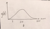
Great! I can use the Distribution Explorer to choose a reasonable prior based on my sketch. I will choose:

\begin{align} g(\phi) \sim \text{Norm}(20, 20). \end{align}

We can plot the result.

phi = np.linspace(-50, 100, 200)
p = bokeh.plotting.figure(
    frame_width=300, frame_height=200, x_axis_label="φ (µm)", y_axis_label="g(φ)"
)
p.line(phi, st.norm.pdf(phi, 20, 20), line_width=2)
bokeh.io.show(p)

For \(g(\sigma)\), I might choose a normal prior again. I think spindle size may vary a fair amount. They are created spontaneously in a droplet, so I would guess there could be many sizes. Therefore, I might choose

\[\begin{aligned} g(\sigma) \sim \text{Norm}(5, 5) \end{aligned}\]

sigma = np.linspace(-10, 20, 100)
p = bokeh.plotting.figure(
    frame_width=300,
    frame_height=200,
    x_axis_label="sigma (µm)",
    y_axis_label="g(sigma)",
)
p.line(sigma, st.norm.pdf(sigma, 5, 5), line_width=2)
bokeh.io.show(p)

In this case, I chose the shape for the prior above because 1) I am speculating that the average length might vary by 25-70%, and 2) this standard deviation is likely to have a distribution that has the shape of a normal distribution.

Visualizing the Prior

The prior can be a bit confusing because it’s hard to think about what it means. When choosing priors, we think about our knowledge of the parameter before collecting data. From what we know, we can estimate the probability of the parameter taking on certain values, and therefore can choose a reasonable distribution for our prior probability. One question that came up in recitation a lot is: what does each part of the prior mean? For example, what does the µ in \(g(\phi) \sim \text{Normal}(\mu, \sigma)\) represent? What about the \(\sigma\)?

Consider our prior \(g(\phi) \sim \text{Normal}(\mu, \sigma)\). We want to choose a prior for \(\phi\) that represents the probability of \(\phi\) taking on possible values. We chose a normal prior, so we are concerned with prior parameters \(\mu\) and \(\sigma\). It is important to note that the \(\mu\) in \(g(\phi) \sim \text{Normal}(\mu, \sigma)\) is not the same parameter as the \(\phi\) in \(l_i \sim \text{Norm}(\phi, \sigma) \;\;\forall i\). In the likelihood, \(l_i \sim \text{Norm}(\phi, \sigma) \;\;\forall i\), \(\phi\) is the location parameter of the PDF of the likelihood, and therefore represents the center of the probability distribution of the values of \(l_i\). In the prior for \(\phi\), \(g(\phi) \sim \text{Normal}(\mu, \sigma)\), \(\mu\) is the location parameter of the probability distribution of the possible values of \(\phi\), the center we were just talking about. Essentially, \(g(\phi)\) is giving the estimated probability distribution for where \(\phi\) lies.

What can be even more confusing is the \(\sigma\) in \(g(\phi) \sim \text{Normal}(\mu, \sigma)\). This is not related to the \(\sigma\) in \(l_i \sim \text{Norm}(\phi, \sigma) \;\;\forall i\)!! In \(g(\phi) \sim \text{Normal}(\mu, \sigma)\), \(\sigma\) is the scale parameter for our PDF for possible \(\phi\)s. If we want to pick a broad normal prior probability distribution for \(\phi\), then \(\sigma\) will be large.

Possibility #2:

You may be thinking: hold on, \(\phi\) and \(\sigma\) could not physically have negative values, so why are we using normal priors that could potentially take on negative values? Totally fair point! We can resolve this in a few ways:

1. If the location parameter for our Normal prior is far away from 0, negative values have a very low probability anyway due to the light tails, so we won’t have to worry about them too much. We can just include a conditional statement in our model to avoid negative values for our prior.

2. We could choose a Log-Normal or Half-Normal prior to avoid this issue. Be sure to review those distributions on the distribution explorer to make sure they are reasonable choices.

Rethinking my prior \(g(\phi)\), I might consider a Log-Normal prior. 1) The Log-Normal prior will not take on negative values, which is physically true for \(\phi\), and 2) I think it is reasonable that \(\text{ln}(\phi)\) is normally distributed. I could expect the probability on the left side of \(\mu\) to vanish more quickly than on the right. So, I will choose:

\begin{align} g(\phi) \sim \text{LogNorm}(\text{ln} \ 20, 0.75) \end{align}

Which looks like:

phi = np.linspace(0, 100, 200)
p = bokeh.plotting.figure(
    frame_width=300, frame_height=200, x_axis_label="phi (µm)", y_axis_label="g(phi)"
)
p.line(phi, st.lognorm.pdf(phi, 0.75, loc=0, scale=20), line_width=2)
bokeh.io.show(p)

Looks reasonable!

Revisiting \(g(\sigma)\), we know it doesn’t make sense for \(\sigma\) to be negative. I think Half-Normal would be an appropriate choice here, especially considering our original plot of \(g(\sigma) \sim \text{Norm}(5, 5)\). It also doesn’t make sense that \(\text{ln}(\sigma)\) would be normally distributed, so Half-Normal is a good choice. I might choose Half-Normal centered at 0 with a large scale parameter, such as

\[\begin{aligned} g(\sigma) \sim \text{HalfNorm}(0, 10) \end{aligned}\]

This would look like:

sigma = np.linspace(0, 40, 200)
p = bokeh.plotting.figure(
    frame_width=300,
    frame_height=200,
    x_axis_label="sigma (µm)",
    y_axis_label="g(sigma)",
)
p.line(phi, st.halfnorm.pdf(sigma, 0, 10), line_width=2)
bokeh.io.show(p)

So, our final model would be:

Possibility #3: A New Model

Let’s use a new model for spindle length where droplet diameter is related to spindle length. To understand how we came up with this model, and its caveats, please refer to the discussion of the model from last term. Be sure to read through this first, otherwise the following will not make sense.

We have a theoretical model relating the droplet diameter to the spindle length. Let us now build a generative model. For spindle, droplet pair i, we assume

\begin{align} l_i = \frac{\gamma d_i}{\left(1+(\gamma d/\phi)^3\right)^{\frac{1}{3}}} + e_i. \end{align}

We will assume that \(e_i\) is Normally distributed with variance \(\sigma^2\). This leads us to our statistical model.

\begin{align} &\mu_i = \frac{\gamma d_i}{\left(1+(\gamma d_i/\phi)^3\right)^{\frac{1}{3}}}, \\[1em] &l_i \sim \text{Norm}(\mu_i, \sigma) \;\forall i, \end{align}

where

\begin{align} \gamma &= \left(\frac{T_0-T_\mathrm{min}}{k^2T_\mathrm{s}}\right)^\frac{1}{3} \\ \phi &= \gamma\left(\frac{6\alpha\beta}{\pi}\right)^{\frac{1}{3}}, \end{align}

which is equivalently stated as

Yikes, we have a lot more parameters in this model! Not to worry, we will choose priors for one parameter at a time. Starting with \(\phi\), this still represents the location parameter for the distribution of spindle size. So, we will use the same prior:

\begin{align} \phi \sim \text{LogNorm}(\mathrm{ln} 20, 0.75) \end{align}

Now let’s consider \(\gamma\). \(\gamma\) determines the relationship between \(d\), the droplet diameter, and \(\phi\), the spindle length. We can already think of some bounds on \(\gamma\). \(\gamma\) must be greater than 0. Also, \(\gamma\) must be less than or equal to 1, or else the spindle length exceeds the droplet diameter. Further, we can see that for large droplets, with \(d \gg \phi/\gamma\), the spindle size becomes independent of \(d\), with

\begin{align} l \approx \phi. \end{align}

Conversely, for $ d \ll `:nbsphinx-math:phi`/:nbsphinx-math:`gamma`$, the spindle length varies approximately linearly with diameter.

\begin{align} l(d) \approx \gamma\,d. \end{align}

Of course, these cases are physically possible. Please see the notes I referenced from BE/Bi 103a to review the limitations of this model. So, we know our model will only work in cases of droplets with intermediate diameter. Thus, we will choose:

\begin{align} \gamma \sim \text{Beta}(2, 2). \end{align}

Let’s take a look.

gamma = np.linspace(0, 1, 100)
p = bokeh.plotting.figure(
    frame_width=300,
    frame_height=200,
    x_axis_label="γ (µm)",
    y_axis_label="γ(gamma)",
    x_range=[0, 1],
)
p.line(gamma, st.beta.pdf(gamma, 2, 2), line_width=2)
bokeh.io.show(p)

Notice how useful the beta distribution can be!

Next, we will consider \(\sigma\). We could use our previous choice, \(\sigma \sim \text{HalfNorm}(0, 10)\). We could also consider the case where we assume \(\sigma\) scales with \(\phi\). This is not an unreasonable assumption. As \(\phi\) increases, we may expect the standard deviation \(\sigma\) to increase as well. We can write the expression:

\begin{align} \sigma = \sigma_0 \phi \end{align}

We have now introduced a new prior parameter, \(\sigma_0\). \(\sigma_0\) is our constant of proportionality for the relationship between \(\sigma\) and \(\phi\). We choose a gamma prior for \(\sigma_0\):

\begin{align} \sigma_0 = \text{Gamma}(2, 10) \end{align}

Gamma makes sense in this case because, as stated in the Distribution Explorer: “it imparts a heavier tail than the Half-Normal distribution (but not too heavy; it keeps parameters from growing too large), and allows the parameter value to come close to zero.” We want to leave room for the case where \(\sigma_0\) is small, so a Gamma distribution is appropriate.

Let’s plot it up to take a look.

sigma_0 = np.linspace(0, 2, 100)
p = bokeh.plotting.figure(
    frame_width=300, frame_height=200, x_axis_label="σ₀", y_axis_label="g(σ₀)"
)
p.line(sigma_0, st.gamma.pdf(sigma_0, 2, loc=0, scale=0.1), line_width=2)
bokeh.io.show(p)

We have now finished building the model:

\begin{align} &\phi \sim \text{LogNorm}(\ln 20, 0.75),\\[1em] &\gamma \sim \text{Beta}(2, 2), \\[1em] &\sigma_0 \sim \text{Gamma}(2, 10),\\[1em] &\sigma = \sigma_0\,\phi,\\[1em] &\mu_i = \frac{\gamma d_i}{\left(1+(\gamma d_i/\phi)^3\right)^{\frac{1}{3}}}, \\[1em] &l_i \sim \text{Norm}(\mu_i, \sigma) \;\forall i. \end{align}

Example 2: Microtubule Catastrophe - Try it yourself!

Dataset download

Gardner, Zanic, and coworkers investigated the dynamics of microtubule catastrophe, the switching of a microtubule from a growing to a shrinking state. In particular, they were interested in the time between the start of growth of a microtubule and the catastrophe event. They monitored microtubules by using tubulin (the monomer that comprises a microtubule) that was labeled with a fluorescent marker. As a control to make sure that fluorescent labels and exposure to laser light did not affect the microtubule dynamics, they performed a similar experiment using differential interference contrast (DIC) microscopy. They measured the time until catastrophe with labeled and unlabeled tubulin.

df_mt = pd.read_csv(
    os.path.join(data_path, "gardner_time_to_catastrophe_dic_tidy.csv"), index_col=0
)
labeled = df_mt.loc[df_mt["labeled"], "time to catastrophe (s)"].values

df_mt.head()

	time to catastrophe (s)	labeled
0	470.0	True
1	1415.0	True
2	130.0	True
3	280.0	True
4	550.0	True

ECDF of Catastrophe Times for Labeled Tubulin

p = iqplot.ecdf(labeled, q='t (s)', conf_int=True)

bokeh.io.show(p)

Last term, we explored a Gamma model for this dataset, which gives the amount of time we have to wait for \(\alpha\) arrivals of a Poisson process. This models a multistep process where each step happens at the same rate. So \(\alpha\) is the number of arrivals, and \(\beta\) is the rate of arrivals.

In the distribution explorer, it is easier to see the impacts of changing the parameters. When \(\beta\) is small, the gamma distribution gets broad. This makes sense because the rate is small and thus the waiting time will likely be larger or more variable. When \(\beta\) rate is large, the gamma distribution gets sharp; the waiting time will be short with a large rate.

We have two parameters - \(\alpha\) and \(\beta\). Let’s try to pick reasonable priors for \(\alpha\) and \(\beta\).

For \(\beta\), we know that it is not physically possible for it to be negative or zero. We also know it will not be faster than the speed of light, ~ 3e8 m/s. In scipy, the lognormal pdf takes in a scale parameter, which is 1/\(\beta\). It might be easier to think of a prior for 1/\(\beta\), instead of \(\beta\) itself. We can define \(\theta\) = 1/\(\beta\). If \(\beta\) is very large, say approaching the speed of light, then \(\theta\) will be very small, approaching zero.

I am not a biologist, but I would bet to say it is unlikely that microtubule catastrophe will take longer than one hours = 3600 seconds. 1/3600 ~ 2e-4 \(\beta\) rate. So we could use 1/2e-4 = 5000 for a \(\theta\) upper bound.

The range 0 – 5000 is a pretty wide, but we could use a lognormal, since I expect more probability towards faster rates than really slow ones. Let’s use a mean of 500.

theta = np.linspace(0, 5000, 200)
p = bokeh.plotting.figure(
    frame_width=400, frame_height=300, x_axis_label="θ (s)", y_axis_label="g(θ)"
)
p.line(theta, st.lognorm.pdf(theta, 0.7, loc=0, scale=500), line_width=2)
bokeh.io.show(p)

For \(\alpha\), we do have a rough bound. We know \(\alpha\) must not be negative, or zero. We also know that if we use a mean \(\theta\) of 500, then \(\beta\) = 1/500 = .002. And, looking at the data, a mean catastrophe time is about 500. If we then use the mean moment of the gamma distribution, and set 500 = \(\alpha\)/ \(\beta\) = \(\alpha\)/ .002, we get an order of magnitude estimate for \(\alpha\) of 1. Based on this, it is not likely to be larger than 10.

alpha = np.linspace(0, 20, 200)
p = bokeh.plotting.figure(
    frame_width=300, frame_height=200, x_axis_label="α", y_axis_label="g(α)"
)
p.line(alpha, st.halfnorm.pdf(alpha, 0, 5), line_width=2)
bokeh.io.show(p)

Computing environment

%load_ext watermark
%watermark -v -p numpy,pandas,bokeh,iqplot,jupyterlab

CPython 3.8.5
IPython 7.19.0

numpy 1.19.2
pandas 1.2.1
bokeh 2.2.3
iqplot 0.2.0
jupyterlab 2.2.6