R9: Sampling discrete parameters with Stan

This recitation was written by Julian Wagner.

---

# Colab setup ------------------
import os, sys, subprocess
if "google.colab" in sys.modules:
    cmd = "pip install --upgrade colorcet bebi103 arviz cmdstanpy watermark"
    process = subprocess.Popen(cmd.split(), stdout=subprocess.PIPE, stderr=subprocess.PIPE)
    stdout, stderr = process.communicate()
    import cmdstanpy; cmdstanpy.install_cmdstan()
    data_path = "https://s3.amazonaws.com/bebi103.caltech.edu/data/"
else:
    data_path = "../data/"
# ------------------------------

import numpy as np
import scipy.special
import pandas as pd

import bebi103

import bokeh
import bokeh.io
import iqplot

import cmdstanpy
import arviz as az

bokeh.io.output_notebook()

Loading BokehJS ...

---

Throughout the term, we have used Stan to great effect to sample from our bespoke statistical models. However, one caveat of the Hamiltonian Monte Carlo is that it can only sample continuous parameters because it relies on concepts of classical mechanics. Fortunately, our old friend marginalization allows us to get around this limit of HMC and handle discrete parameters in our models. This notebook has a few examples of how to handle discrete variables in Stan: one from the ecological realm of mark and recapture experiments, and one from a simulated dataset based on one of the hypothetical experiments in HW6.1. I heavily relied on the materials on handling latent discrete parameters in the Stan language reference in prepping these materials.

Review of LogSumExp, the cornerstone of stable marginalization with discrete parameters

---

Before we jump into sampling discrete parameters in Stan, I will first review the LogSumExp trick, which we will use over and over while dealing with discrete parameters. I found a couple of blog posts here and here helpful when thinking about the LogSumExp operation. What is LogSumExp? It is a nifty operation that makes the addition of a series of numbers more numerically stable. In particular, consider a situation where we are interested in calculating \(y\), with \begin{align} y = \mathrm{log}\sum_{i=1}^{n}\mathrm{exp}(x_i). \end{align} We will see in a moment why this comes up in dealing with discrete parameters. We can take \(\mathrm{exp}\) of both sides of the equation to give \begin{align} \mathrm{exp}(y) = \sum_{i=1}^{n}\mathrm{exp}(x_i). \end{align} We can now multiply both sides by a constant, say \(\mathrm{exp}(-a)\) \begin{align} \mathrm{exp}(-a) \cdot \mathrm{exp}(y) = \mathrm{exp}(-a) \cdot \sum_{i=1}^{n}\mathrm{exp}(x_i). \end{align} We rearrange the expression to give \begin{align} \mathrm{exp}(y-a) = \sum_{i=1}^{n}\mathrm{exp}(x_i-a). \end{align} Then we can take the \(\mathrm{log}\) of both sides, giving \begin{align} y-a = \mathrm{log} \sum_{i=1}^{n}\mathrm{exp}(x_i-a). \end{align} We can then rearrange to give \begin{align} y = a + \mathrm{log} \sum_{i=1}^{n}\mathrm{exp}(x_i-a). \end{align}

Nice, so we can subtract a constant from each data point \(x_i\) before we exponentiate, sum, and take the log, so long as we add it back afterwards. This is referred to as the LogSumExp trick; in particular, we take \(a\) to be the max of \(x_i\) when performing the computation. This operation makes it much less likely to encounter over or underflow problems while doing the computation. The maximal value that we end up with after subtracting the \(\mathrm{max}(x_i)\) is 0, and \(\mathrm{exp}(0)=1\). The worst case scenario, where every result of the exponentiation operation save the max value of \(x_i\) (which gives 1 by definition) results in underflow (0 for every other term), we still have log(1) for the sum term, which means we will not get the dreaded nan from this term. Instead, y will simply be determined by the \(\mathrm{max}(x_i)\). While this wouldn’t necessarily be an ideal situation, y would still approximate the true value of the sum (if we were able to calculate it without running out of storage space for our datatype), and is nicely behaved instead of exploding our numerics. If we don’t do the trick and every single term results in underflow, we instead will encounter \(\mathrm{log}(0)\), which is nan, and kills that whole iteration of the computation.

Handling log probabilities of discrete valued vectors in Stan

A need to quantifying the size of natural populations of animals often arises in ecology. A popular approach to count populations is to mark them with a label of some type like a leg bands on a birds or a fin tags on a shark. In 1970, Stradling marked ants by feeding them with radioactive phosphorous (32P), which would get integrated into their tissue and persist over time without transferring to their other ants.

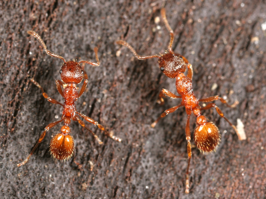
Worker Myrmica rubra ants. Image by Gary Alpert, can be found here

After labeling a bunch of animals, Stradling released them back into the population and allowed them to mix. Then, he re-sampled and counted how many of the labeled animals he pulled from the population. As an introduction to the concepts used in handling discrete parameters, I will first code up how to quantify the population size based on this information in Stan (a brute force type approach) before mixing in continuous variables with some other mark and recapture data. It is quite apparent that Stradling’s data matches the story of the hypergeometric distribution. We will call the radioactively labeled ants the ‘white balls’, and the unlabeled ones the ‘black balls’, which are mixed together in the colony and then samples without replacement. Hence, we have

\begin{align} n &\sim \text{hypergeometric}(N, a, b) \end{align}

Where \(N\) is the number of animals sampled from the mixed labeled-unlabeled population, \(n\) is the number of labeled animals drawn, \(a\) is the number of animals labeled before release, and \(b\) is the number of unlabeled animals. With this formulation, the population size of ants in a colony is given by \(a+b\). We could get a very good approximation of this with the Binomial distribution most of the time, i.e. we look at the success rate \(\theta\) of drawing a marked individual and use that as a ratio of marked to total population to get the answer. This would probably work well since ant populations are often pretty large, as are the number of ants labeled and sampled, but we are going to be sticklers today and insist that we use discrete quantities. Now we need to think about a prior for \(b\) to finish building the model. Since we are sticking with discrete, I chose a negative binomial, since it can be shaped as a broad/peaked distribution.

\begin{align} b &\sim \text{negative binomial}(\mu=1000, \phi=2) \end{align}

We can do a quick prior predictive check in numpy to see how this looks. For this, we will assume an experimental design where 100 animals were marked to begin, and the subsequent recaptures are also of 100 individuals.

a = 100
N = 100
n = []
for i in range(1000):
    b = np.random.negative_binomial(2, 2/(1000+2))
    n.append(np.random.hypergeometric(a, b, N))

bokeh.io.show(iqplot.ecdf(np.array(n)))

This makes sense: the prior allows the population to be nearly all included in the initial sample of 100 animals, or could be much bigger, in which case the number of animals re-captured goes towards 0. Looking back, this model doesn’t even have any continuous parameters at all! What can Stan possibly bring to the table? Well, it would clearly be quite easy to brute force plot the posterior for \(b\) as we did for the worm reversal probability in a the HW (seems like ages ago!). We can do a similar thing in Stan, taking advantage of it’s built in log pmf functions, and it’s nifty log_sum_exp function. Basically, the name of the game is to decide a range of values for \(b\) that we will look at, evaluate the model at all these values, and plot the result. Note that we know the value for \(b\) must be at least as large as \(N\)-\(n\) (the number of animals that were not marked in our re-sample).

sm = cmdstanpy.CmdStanModel(stan_file='mark_recapture_hypergeometric.stan')
print(sm.code())

INFO:cmdstanpy:compiling stan program, exe file: /Users/bois/Dropbox/git/bebi103_course/2021/b/content/recitations/09/mark_recapture_hypergeometric
INFO:cmdstanpy:compiler options: stanc_options=None, cpp_options=None
INFO:cmdstanpy:compiled model file: /Users/bois/Dropbox/git/bebi103_course/2021/b/content/recitations/09/mark_recapture_hypergeometric

data {
  // Measured data
  int a;
  int N;
  int n;
  int max_pop;
  int min_pop;
  real mu;
  real phi;

}

transformed data{
  int b[max_pop-min_pop];
  for(i in 1:max_pop-min_pop){
    b[i] = i+min_pop;
  }
}

transformed parameters{
  vector[max_pop-min_pop] lp;
  for(i in 1:max_pop-min_pop){
    lp[i] = neg_binomial_2_lpmf(b[i]|mu, phi) + hypergeometric_lpmf(n|N, a, b[i]);
  }
}


model {
  target += log_sum_exp(lp);
}

generated quantities{
  simplex[max_pop-min_pop] pState;
  int num[max_pop-min_pop];
  num = b;
  pState = exp(lp - log_sum_exp(lp));

}

The only other bit of funny business is going on in the generated quantities block. We are taking our unnormalized probability for \(b\) and normalizing it based on averaging over log posterior draws for a given discrete value, which marginalizes them out. In this case, we don’t have continuous parameters, but we are still normalizing based on the marginalized posterior probability. Let’s give this a spin and see what it yields! I will manually input some data from Stradling’s paper here to test with.

a = 190
N = 346
n = 32

#a = 17
#N = 33
#n = 13

#a = 308
#N = 279
#n = 186

data = {
    'a': a,
    'N': N,
    'n': n,
    'max_pop': 4000,
    'min_pop': N-n,
    'mu': 1000.0,
    'phi': 2.0
}

Note that since we don’t have any model parameters, we must run the sampler with fixed_param=True. Also, we only need 1 for sample_iters since the calculations performed in the Stan code are deterministic (we aren’t actually sampling).

samples = az.from_cmdstanpy(sm.sample(data=data, fixed_param=True, iter_sampling=1))

INFO:cmdstanpy:start chain 1
INFO:cmdstanpy:finish chain 1

For plotting the results, note that I am showing \(b+a\), as \(b\) represents the number of unlabeled ants and \(a\) is the number of labeled, so \(b+a\) is the total population size.

p = bokeh.plotting.figure(
    plot_height=300,
    x_axis_label="number of ants in colony",
    y_axis_label="posterior probability",
    title="Distibution of ant colony size given data",
)
p.scatter(
    samples.posterior["num"].values[0][0] + a, samples.posterior["pState"].values[0][0]
)
bokeh.io.show(p)

As a last check to make sure we properly generated our posterior probability values here, we will do a quick numerical integration on the posterior above. This should give a value of 1 for the area under our posterior, since it is a probability distribution.

np.trapz(samples.posterior['pState'].values[0][0], samples.posterior['num'].values[0][0]+a)

1.0000000284678414

Yay, it is a probability distribution! This seems like a lot of work for where we’ve gotten! Though we have not yet sampled a model with both discrete and continuous parameters, this gives us all the building block we need in order to do so.

Discrete paremeters in Stan: integer α for gamma distribution

We will build a model for experiment 5 from HW 6.2. Recall the description:

Experiment 5: You are studying a signaling pathway that, when the ligand binds the receptor, forms a multimeric protein complex at the intracellular side of the membrane. You assume that the rate of each protein joining this complex is roughly the same. You want to estimate the number of proteins in this complex, and the average rate at which they join. You employ a similar approach as in Experiment 3, using protein fusions that produce a fluorescent signal only when the complex is fully-formed. You use time-lapse microscopy to time how long it takes the complex to fully form after you add the ligand.

Although we always prefer to use real data in this class, we will simulate this process for the sake of time for this recitation. We will assume that the process is described by 3 arrivals of a Poisson process with the same arrival rate parameter. To simulate the experiment, we will make 50 data points of arrival times measured from the time-lapse microscope modeled as the sum of the arrival time of 3 successive and identical exponential distributions.

al = 3
ra = 0.5
t = np.zeros(50)

for i in range(al):
    t += np.random.exponential(1 / ra, size=len(t))

We can now take a look at what the simulated data looks like

p = iqplot.ecdf(t, x_axis_label='time fully formed complex')
bokeh.io.show(p)

With this in hand, we first apply a model that we know well: a gamma distribution as in the microtubule catastrophe data. Our model is as follows

\begin{align} \alpha &\sim \text{HalfNorm}(0, 3) \\ \beta &\sim \text{HalfNorm}(0, 10) \\ t_i &\sim \text{gamma}(\alpha, \beta) \, \forall i \end{align}

Great, with the model defined we can prepare our data, compile the model, and print the Stan code.

data = {"t": t, "N": len(t), "a_min": 0, "a_max": 10}

sm = cmdstanpy.CmdStanModel(stan_file="mt_gamma.stan")
print(sm.code())

INFO:cmdstanpy:compiling stan program, exe file: /Users/bois/Dropbox/git/bebi103_course/2021/b/content/recitations/09/mt_gamma
INFO:cmdstanpy:compiler options: stanc_options=None, cpp_options=None
INFO:cmdstanpy:compiled model file: /Users/bois/Dropbox/git/bebi103_course/2021/b/content/recitations/09/mt_gamma

data {
  int N;
  real t[N];
}


parameters {
  real<lower=0> alpha;
  real<lower=0> beta_;
}


model {
  alpha ~ normal(0, 3);
  beta_ ~ normal(0, 10);

  t ~ gamma(alpha, beta_);
}


generated quantities {
  real t_ppc[N];

  for (i in 1:N) {
    t_ppc[i] = gamma_rng(alpha, beta_);
  }
}

We are now ready to sample!

samples = az.from_cmdstanpy(sm.sample(data=data, iter_sampling=20000), posterior_predictive="t_ppc")

INFO:cmdstanpy:start chain 1
INFO:cmdstanpy:start chain 2
INFO:cmdstanpy:start chain 3
INFO:cmdstanpy:start chain 4
INFO:cmdstanpy:finish chain 3
INFO:cmdstanpy:finish chain 1
INFO:cmdstanpy:finish chain 4
INFO:cmdstanpy:finish chain 2

We now check the diagnostics.

print(f"\nDiagnostics for gamma...")
bebi103.stan.check_all_diagnostics(samples)

Diagnostics for gamma...
Effective sample size looks reasonable for all parameters.

Rhat looks reasonable for all parameters.

0 of 80000 (0.0%) iterations ended with a divergence.

0 of 80000 (0.0%) iterations saturated the maximum tree depth of 10.

E-BFMI indicated no pathological behavior.

0

We take a look at the posterior predictive distribution

t_ppc = (
    samples.posterior_predictive["t_ppc"]
    .stack({"sample": ("chain", "draw")})
    .transpose("sample", "t_ppc_dim_0")
)

bokeh.io.show(
    bebi103.viz.predictive_ecdf(
        t_ppc,
        data=t,
        title="Gamma",
        diff="ecdf",
        x_axis_label='time fully formed complex',
    )
)

We can see how the model parameters correspond to our known parameter values used to produce the data.

bokeh.io.show(bebi103.viz.corner(samples, xtick_label_orientation=np.pi / 4))

These don’t look bad, but it is pretty unsatisfying that we get an alpha value between 2 and 3, given that we know the underlying process must have an integer for \(\alpha\). We can implement this model explicitly by marginalizing over discrete values of \(\alpha\). This model is below.

Take two: handling discrete parameters via marginalization

---

Let us suppose that instead of allowing \(\alpha\) to take on a continuous range of values, that we instead consider it as a discrete parameter. We can select a discrete prior for \(\alpha\), and leave the rate parameter \(\beta\) as continuous. The model we will consider is as follows \begin{align} &\alpha_{max} = 7 \\[1em] &\alpha \sim \text{Binomial}(\alpha_{max}, 0.5) \\[1em] &\beta \sim \text{HalfNorm}(0, 1) \\[1em] &t_j \sim \text{gamma}(\alpha, \beta) \, \forall j \end{align}

Note that the selection of \(\alpha\) prior forces the parameter to be in discrete, and in [0, 1, …, \(\alpha_{max}\)]. How are we to handle this parameter in Stan? We need to marginalize this parameter out, and then sample \(\beta\) via the usual MCMC approach. We will be able to draw samples for the \(\alpha\) parameter based on the probability of the various possible values of \(\alpha\) given when we marginalize it out of the posterior. To make the planned procedure more concrete, I will write out Bayes’ theorem for our model.

\begin{align} g(\alpha, \beta \, | \, \{t_j\}) \propto \left[ \prod_{j=1}^{n} f(t_j \,|\, \alpha, \beta)\right]g(\alpha)g(\beta). \end{align}

We can marginalize out \(\alpha\) to get an expression for \(g(\beta \, | \, \{t_j\})\). Note that since \(\alpha \in [0, 1, ... , \alpha_{max}]\), all we need to do to marginalize is sum over all these values of \(\alpha\). The expression for this is

:nbsphinx-math:`begin{align} g(beta , | , {t_j}) &propto sum_{i=1}^{a_{max}} left[ prod_{j=1}^{n} f(t_j ,|, alpha_i, beta)right]g(alpha_i)g(beta) \

& = g(beta)sum_{i=1}^{a_{max}} left[ prod_{j=1}^{n} f(t_j ,|, alpha_i, beta)right]g(alpha_i)

end{align}`

In Stan, we always work with log values, so the expression we will be working with is \begin{align} \text{log} \, g(\beta \, | \, \{t_j\}) &\propto \text{log} \, g(\beta) + \text{log} \, \sum_{i=1}^{a_{max}} \left[ \prod_{j=1}^{n} f(t_j \,|\, \alpha_i, \beta)\right]g(\alpha_i) \end{align}

To help with numerical stability, we also want to work with the log of the of the product components. To do this, we can consider \(\mathrm{exp}(\mathrm{log}(\text{product}))\). That is, we consider

:nbsphinx-math:`begin{align}

&text{log} , g(beta) + text{log} , sum_{i=1}^{a_{max}} left[ prod_{j=1}^{n} f(t_j ,|, alpha_i, beta)right]g(alpha_i) \ = , &text{log} , g(beta) + text{log} , sum_{i=1}^{a_{max}} mathrm{exp}left( mathrm{log} , prod_{j=1}^{n} f(t_j ,|, alpha_i, beta)g(alpha_i)right) \ = , &text{log} , g(beta) + text{log} , sum_{i=1}^{a_{max}} mathrm{exp}left(mathrm{log} , g(alpha_i) + sum_{j=1}^{n} mathrm{log} , f(t_j ,|, alpha_i, beta)right)

end{align}`

Hey, look at that second term! It is exactly the form of function that we can apply the LogSumExp trick to. This is why LogSumExp is so important for dealing with the discrete parameters; is is the numerically stable approach we can use to marginalize out the discrete parameter. I will first define the Stan model below, and then give a bit more explanation of the components.

sm2 = cmdstanpy.CmdStanModel(stan_file="mt_gamma_integer_alpha.stan")
print(sm2.code())

INFO:cmdstanpy:compiling stan program, exe file: /Users/bois/Dropbox/git/bebi103_course/2021/b/content/recitations/09/mt_gamma_integer_alpha
INFO:cmdstanpy:compiler options: stanc_options=None, cpp_options=None
INFO:cmdstanpy:compiled model file: /Users/bois/Dropbox/git/bebi103_course/2021/b/content/recitations/09/mt_gamma_integer_alpha

data {
  int N;
  real t[N];
  int a_min;
  int a_max;
}


transformed data{
  int a[a_max-a_min];
  for(i in 1:a_max-a_min){
    a[i] = i+a_min;
  }
}

parameters {
  real<lower=0> beta_;
}

transformed parameters {
  real<lower=0> beta2 = beta_;
  vector[a_max-a_min] lp;
  for(i in 1:a_max-a_min){
    lp[i] = binomial_lpmf(a[i]|a_max, 0.5);
    for(j in 1:N){
      lp[i] = lp[i] + gamma_lpdf(t[j]|a[i],beta_);
    }
  }
}

model {
  beta_ ~ normal(0, 1);
  target += log_sum_exp(lp);
}


generated quantities {
  real t_ppc[N];
  simplex[a_max-a_min] pState;
  int num[a_max-a_min];
  vector[a_max-a_min] log_p_norm;
  num = a;
  log_p_norm = lp - log_sum_exp(lp);
  pState = exp(log_p_norm);

  real alpha = categorical_logit_rng(log_p_norm);
  for (i in 1:N) {
    t_ppc[i] = gamma_rng(alpha, beta_);
  }

}

There are a couple of notable differences in how we implement this model as compared to our usual Stan models. For one, we do the heavy lifting of the marginalization of the discrete parameter via the transformed parameters block. We store the log of the the terms inside the \(\mathrm{exp}\) of the expression we wrote above. We then compute the LogSumExp of the terms in that vector in the model block and add to the target. Recall that the target variable is where the log posterior value is stored in Stan. The other strange bit of code is in the generated quantities block. In this block, we are getting actual samples for the discrete \(\alpha\) that we had marginalized out. The strategy to do this is to use the log joint values we calculated in the transformed parameters block to perform a second round of marginalization (via the LogSumExp) to calculate the evidence term from Bayes’ theorem and calculate probability values for each of the discrete parameter values that \(\alpha\) can take on given the current value of the \(\beta\) parameter. If we know the probability of each potential \(\alpha\) value (or log probability) we can draw a sample from that probability distribution using a categorical rng, or, equivalently, a categorical logit rng. With a sample for both the \(\alpha\) and the \(\beta\), we can do posterior predictive checks just as we would with any other model.

One caveat of this modeling approach is that we must decide what range of values to look at our discrete parameter. Usually, if we are planning on using a discrete model for a process, we probably have at least fairly strong opinions about what the parameter value should approximately look like. For our case, I am forcing an upper limit on the parameter value by my choice of prior as a Binomial distribution. Let’s sample!

data = {"t": t, "N": len(t), "a_min": 0, "a_max": 7}
samples_discrete = az.from_cmdstanpy(
    sm2.sample(data=data, iter_sampling=20000), posterior_predictive="t_ppc"
)

INFO:cmdstanpy:start chain 1
INFO:cmdstanpy:start chain 2
INFO:cmdstanpy:start chain 3
INFO:cmdstanpy:start chain 4
INFO:cmdstanpy:finish chain 4
INFO:cmdstanpy:finish chain 3
INFO:cmdstanpy:finish chain 1
INFO:cmdstanpy:finish chain 2

We check the diagnostics.

bebi103.stan.check_all_diagnostics(samples_discrete, parameters=['beta_'])

Effective sample size looks reasonable for all parameters.

Rhat looks reasonable for all parameters.

0 of 80000 (0.0%) iterations ended with a divergence.

0 of 80000 (0.0%) iterations saturated the maximum tree depth of 10.

E-BFMI indicated no pathological behavior.

0

Looks good! Time to take a look at the marginalized posterior for \(\beta\), as well as our samples for \(\alpha\).

p = bebi103.viz.corner(
    samples_discrete, parameters=["beta_", "alpha"], xtick_label_orientation=np.pi / 4, max_plotted=1000
)
bokeh.io.show(p)

Looks a bit odd! Let’s look at an ECDF of the \(\beta\) values.

bokeh.io.show(
    iqplot.ecdf(samples_discrete.posterior.beta_.values.flatten()[::10], x_axis_label="β")
)

Well that looks funky! This is clearly a multi-modal posterior. If you think about the data we generated, this actually makes sense. The value of \(\beta\) depends strongly on how many arrivals we have: fewer arrivals means a slower arrival rate to give a similarly centered distribution. Even so, we can see that some intermediary values of \(\beta\) are preferred here. If you zoom in on the trace plot, you can see the walker shift from peak to peak in this posterior.

bokeh.io.show(
    bebi103.stan.viz.trace(
        samples_discrete, parameters=["beta_"], line_kwargs=dict(line_width=2)
    )
)

Let us take a look at our samples for \(\alpha\).

bokeh.io.show(
    iqplot.ecdf(samples_discrete.posterior["alpha"].values.ravel()[::10], x_axis_label="α")
)

Next, I will compare the samples we got for our discrete model with the ones from the regular gamma model.

df_sample_compare = pd.DataFrame(
    {"samples": samples_discrete.posterior["beta_"].values[0][::10], "cat": "discrete"}
).append(
    pd.DataFrame(
        {"samples": samples.posterior["beta_"].values.ravel()[::10], "cat": "continuous"}
    )
)

p = iqplot.ecdf(df_sample_compare, q="samples", cats="cat")

p.legend.location = "bottom_right"
bokeh.io.show(p)

We can see that the parameter value takes on a similar range of values, though with our discrete model it favors a peaky distribution for the arrival rates governed by the alpha parameter. With a quick predictive ECDF we can confirm that the model offers a similar ability to generate the data.

t_ppc = (
    samples_discrete.posterior_predictive["t_ppc"]
    .stack({"sample": ("chain", "draw")})
    .transpose("sample", "t_ppc_dim_0")
)


p1 = bebi103.viz.predictive_ecdf(
    t_ppc,
    data=t,
    title="Gamma, discrete α",
    diff="ecdf",
    x_axis_label="time fully formed complex",
)

t_ppc = (
    samples.posterior_predictive["t_ppc"]
    .stack({"sample": ("chain", "draw")})
    .transpose("sample", "t_ppc_dim_0")
)

p2 = bebi103.viz.predictive_ecdf(
    t_ppc, data=t, title="Gamma", diff="ecdf", x_axis_label="time fully formed complex",
)
bokeh.io.show(bokeh.layouts.gridplot([p1, p2], ncols=1))

Nice! We can construct a model for discrete values of arrival numbers in a gamma distribution. However, the story doesn’t end here. Notice that there are multiple peaks in the posterior for \(\beta\) in this model. We can see that, due to the fairly small number of data points, there is quite a bit of overlap between the samples given for \(\beta\) for cases of \(\alpha=N\) and \(\alpha=N+1\). This ensures that the sampler is able to explore the posterior, and the chains mix. Here is the posterior again to illustrate this:

p = bebi103.viz.corner(samples_discrete, parameters=["beta_", "alpha"], max_plotted=1000)
bokeh.io.show(p)

This is, however, not necessarily going to be the case. If we had a larger number of data points, for example, the peakiness of the log posterior around a \(\beta\) given by a particular \(\alpha\) increases. As a result, the sampler has a much lower chance of crossing from one peak in the posterior to another. We can simulate this by upping the number of simulated data points and seeing if our model can handle it. We go from 50 to 500 data points.

al = 3
ra = 0.5
t = np.zeros(500)

for i in range(al):
    t += np.random.exponential(1 / ra, size=len(t))

Now we try to sample again.

data = {"t": t, "N": len(t), "a_min": 0, "a_max": 7}

samples_discrete = az.from_cmdstanpy(
    sm2.sample(data=data, iter_sampling=20000, seed=87136123), posterior_predictive="t_ppc"
)

INFO:cmdstanpy:start chain 1
INFO:cmdstanpy:start chain 2
INFO:cmdstanpy:start chain 3
INFO:cmdstanpy:start chain 4
INFO:cmdstanpy:finish chain 3
INFO:cmdstanpy:finish chain 1
INFO:cmdstanpy:finish chain 4
INFO:cmdstanpy:finish chain 2

Time to take a look at the diagnostics.

bebi103.stan.check_all_diagnostics(samples_discrete, parameters=['beta_',])

ESS for parameter beta_ is 7.070924921033623.
ESS / iter for parameter beta_ is 8.83865615129203e-05.
tail-ESS for parameter beta_ is 25.400625192984347.
ESS / iter for parameter beta_ is 0.0003175078149123043.
  ESS or tail-ESS below 100 per chain indicates that expectation values
  computed from samples are unlikely to be good approximations of the
  true expectation values.
  ESS / iter or tail-ESS / iter below 0.001 indicates that the effective
  sample size has likely been overestimated.

Rhat for parameter beta_ is 1.5278465698127859.
  Rank-normalized Rhat above 1.01 indicates that the chains very likely have not mixed.

0 of 80000 (0.0%) iterations ended with a divergence.

0 of 80000 (0.0%) iterations saturated the maximum tree depth of 10.

E-BFMI indicated no pathological behavior.

3

Oh no! These look very bad. We will look at the corner plot to figure out what is going on. We will color by chain to see each chain is doing.

p = bebi103.viz.corner(
    samples_discrete,
    parameters=["beta_", "alpha"],
    max_plotted=1000,
    color_by_chain=True,
)
bokeh.io.show(p)

On face, this looks kind of ok. It looks like we once again have a peaky posterior for \(\beta\). Notice, though, that the sharpness/separation of these peaks is much larger before.

In looking at the colors, the chains are clearly not mixing. Based on this, it seems clear that the sampler is arriving at one peak for \(\beta\) based on where the walker started, and getting stuck there. With a huge number of steps, it might eventually make it over to the other peak, but the odds of that are quite low. This means that we are not sampling from the posterior. What to do about this? Well, we can once again take advantage of marginalization to try a different implementation of a similar approach. For this case, we will sample from \(N\) gamma distributions, each with a set integer value for \(\alpha\). We can then marginalize over the samples to get a value for the probability of a given \(\alpha\) given the model. In this way, we sample from the models independently, so we don’t have to worry about having the sampler make it from one peak to another in the posterior space. We will first sample with the larger dataset, and then compare this model to our previous one with the smaller dataset.

sm = cmdstanpy.CmdStanModel(stan_file='mt_gamma_integer_alpha_jb.stan')
print(sm.code())

INFO:cmdstanpy:compiling stan program, exe file: /Users/bois/Dropbox/git/bebi103_course/2021/b/content/recitations/09/mt_gamma_integer_alpha_jb
INFO:cmdstanpy:compiler options: stanc_options=None, cpp_options=None
INFO:cmdstanpy:compiled model file: /Users/bois/Dropbox/git/bebi103_course/2021/b/content/recitations/09/mt_gamma_integer_alpha_jb

data {
  int N;
  real t[N];

  int alpha;

  int N_ppc;
}


parameters {
  real<lower=0> beta_;
}


model {
  beta_ ~ normal(0, 1);
  t ~ gamma(alpha, beta_);
}


generated quantities {
  real t_ppc[N_ppc];
  real log_lik[N];
  real lp = normal_lpdf(beta_ | 0, 1);
  real log_alpha_prior = binomial_lpmf(alpha|7, 0.5);

  for (i in 1:N_ppc) {
    t_ppc[i] = gamma_rng(alpha, beta_);
  }

  for (i in 1:N) {
    log_lik[i] = gamma_lpdf(t[i] | alpha, beta_);
  }

  lp += sum(log_lik) + log_alpha_prior;
}

This model looks quite a bit simpler than the one we used to marginalize the discrete parameter out. The first blocks look just like a gamma distribution, but note that now \(\alpha\) isn’t a parameter at all. Instead, we are taking \(\alpha\) to be a fixed integer value. The section that needs some explanation is the generated quantities block. We use the generated quantities to calculate the un-normalized log probability of a the current \(\beta\) value given our fixed value of \(\alpha\). This is like what we do to perform model comparison; we generate the pointwise log joint value for every sample iteration. We will use this to generate a probability of a given value of \(\alpha\) in a subsequent Numpy calculation below.

Time to sample!

ms = list(range(1, 8))
N_ppc = len(t)
datas = {m: dict(t=t, N=len(t), alpha=m, N_ppc=N_ppc) for m in ms}

with bebi103.stan.disable_logging():
    samples = {
        m: az.from_cmdstanpy(
            sm.sample(data=datas[m], iter_sampling=3000),
            log_likelihood="log_lik",
            posterior_predictive="t_ppc",
        )
        for m in ms
    }

log_q = np.array(
    [
        scipy.special.logsumexp(samp.posterior.lp.values.flatten())
        - np.log(len(samp.posterior.lp.values.flatten()))
        for m, samp in samples.items()
    ]
)

log_norm_const = scipy.special.logsumexp(log_q)
log_g = log_q - log_norm_const

g = np.exp(log_g)

This all looks very familiar (sampling over a set of models and such), except for the bit at the end where we do some computation on the lp values that we calculated in the generated quantities block. Though it may look odd due to the LogSumExp operation here, what we have actually done when computing log_q is to average the log probability over the samples. What does this accomplish? Since we have drawn samples for the values of \(\beta\), when we compute this average across the samples (hence fully taking into account the parameter \(\beta\)) we are performing marginalization. This means that we are getting an estimate proportional to the log probability of each value for \(\alpha\). To get an actual number for the probability, we need to normalize across our values that are proportional to the log probabilities. This is done with that last set of lines with the application of the logsumexp, subtraction, and exponentiation. The net result of these operations is to give us the marginalized posterior for the parameter \(\alpha\). We can take a look at it!

p = bokeh.plotting.figure(
    frame_height=200,
    frame_width=400,
    x_axis_label='α',
    y_axis_label='g(α | t)'
)

p.circle(ms, g, size=10)

bokeh.io.show(p)

With the larger dataset, the model very heavily favors the known value that we used to generate the data. This is no surprise. We will use the posterior for \(\alpha\) to draw samples for \(\beta\) from the combined model: the probability of drawing \(\beta\) from the samples for a given value of \(\alpha\) is proportional to the posterior probability of \(\alpha\).

betas = [
    np.random.choice(
        samples[np.random.choice(len(g), p=g) + 1].posterior.beta_.values.flatten()[::10]
    )
    for i in range(10000)
]
p = iqplot.ecdf(np.array(betas), x_axis_label="β")
bokeh.io.show(p)

This ends up simply pulling samples from the \(\alpha=3\) case, since this is very much favored by the model. We now return to the smaller dataset and check that our models correspond with each other.

al = 3
ra = 0.5
t = np.zeros(50)

for i in range(al):
    t += np.random.exponential(1 / ra, size=len(t))

Now we try to sample again.

data = {"t": t, "N": len(t), "a_min": 0, "a_max": 7}
samples_discrete = az.from_cmdstanpy(
    sm2.sample(data=data, iter_sampling=20000), posterior_predictive="t_ppc"
)

INFO:cmdstanpy:start chain 1
INFO:cmdstanpy:start chain 2
INFO:cmdstanpy:start chain 3
INFO:cmdstanpy:start chain 4
INFO:cmdstanpy:finish chain 4
INFO:cmdstanpy:finish chain 2
INFO:cmdstanpy:finish chain 1
INFO:cmdstanpy:finish chain 3

Now we sample from our second model implementation.

ms = list(range(1, 8))
N_ppc = len(t)
datas = {m: dict(t=t, N=len(t), alpha=m, N_ppc=N_ppc) for m in ms}

with bebi103.stan.disable_logging():
    samples = {
        m: az.from_cmdstanpy(
            sm.sample(data=datas[m], iter_sampling=3000),
            log_likelihood="log_lik",
            posterior_predictive="t_ppc",
        )
        for m in ms
    }

log_q = np.array(
    [
        scipy.special.logsumexp(samp.posterior.lp.values.flatten())
        - np.log(len(samp.posterior.lp.values.flatten()))
        for m, samp in samples.items()
    ]
)

log_norm_const = scipy.special.logsumexp(log_q)
log_g = log_q - log_norm_const

g = np.exp(log_g)

With these samples in hand, we can compare the posteriors of \(\alpha\), as well as for \(\beta\).

p = bokeh.plotting.figure(
    frame_height=200, frame_width=400, x_axis_label="α", y_axis_label="g(α | t)"
)

p.circle(ms, g, size=10, legend_label="discrete sampling")

for s in range(7):
    p.diamond(
        s + 1,
        samples_discrete.posterior.pState.values[:, :, s].flatten().mean(),
        size=10,
        alpha=1,
        color="red",
        legend_label="separate models",
    )

bokeh.io.show(p)

Nice! These look quite similar to each other. Note that since we are getting these posteriors by marginalizing over samples, they may differ some based on stochasticity in the samples. We now generate some \(\beta\) values from our second model.

betas = [
    np.random.choice(
        samples[np.random.choice(len(g), p=g) + 1].posterior.beta_.values.flatten()
    )
    for i in range(10000)
]

Now we can plot the posterior for \(\beta\).

df_sample_compare = pd.DataFrame(
    {
        "samples": samples_discrete.posterior.beta_.values.flatten()[::10],
        "cat": "discrete sampling",
    }
).append(pd.DataFrame({"samples": np.array(betas), "cat": "separate models"}))

p = iqplot.ecdf(df_sample_compare, q="samples", cats="cat")
p.legend.location = "bottom_right"
bokeh.io.show(p)

These models yield quite similar results for the posteriors! Overall, it seems that working with discrete parameters in a case like this is only useful if we are somewhat data poor or working with an intermediate number of states. At small numbers of arrivals, we see a huge difference in \(\beta\) for a change in \(\alpha\), which makes the posterior for \(\beta\) peaky and impossible to sample. With a large number of arrivals, we would end up with a large range of possible arrival number, which makes it odd to even work with discrete parameters (the continuous approximation doesn’t really lose anything). The computation also becomes monstrous for a large number of possible states. For this type of model, it seems like using discrete sampling is limited in usefulness.

bebi103.stan.clean_cmdstan()

Computing environment

%load_ext watermark
%watermark -v -p numpy,pandas,numba,cmdstanpy,arviz,bebi103,iqplot,jupyterlab

CPython 3.8.8
IPython 7.21.0

numpy 1.19.2
pandas 1.2.3
numba 0.51.2
cmdstanpy 0.9.68
arviz 0.11.1
bebi103 0.1.3
iqplot 0.2.0
jupyterlab 2.2.6