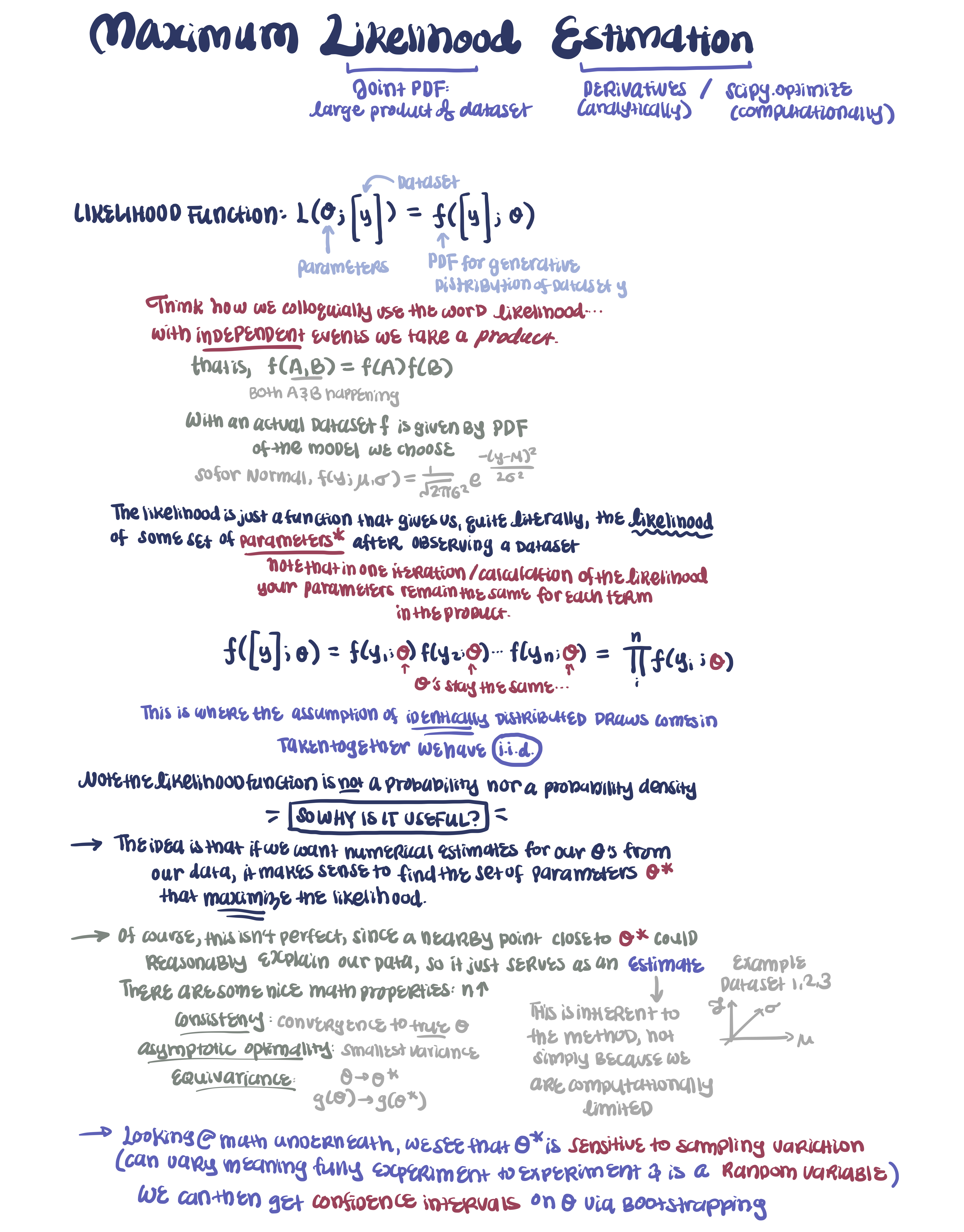
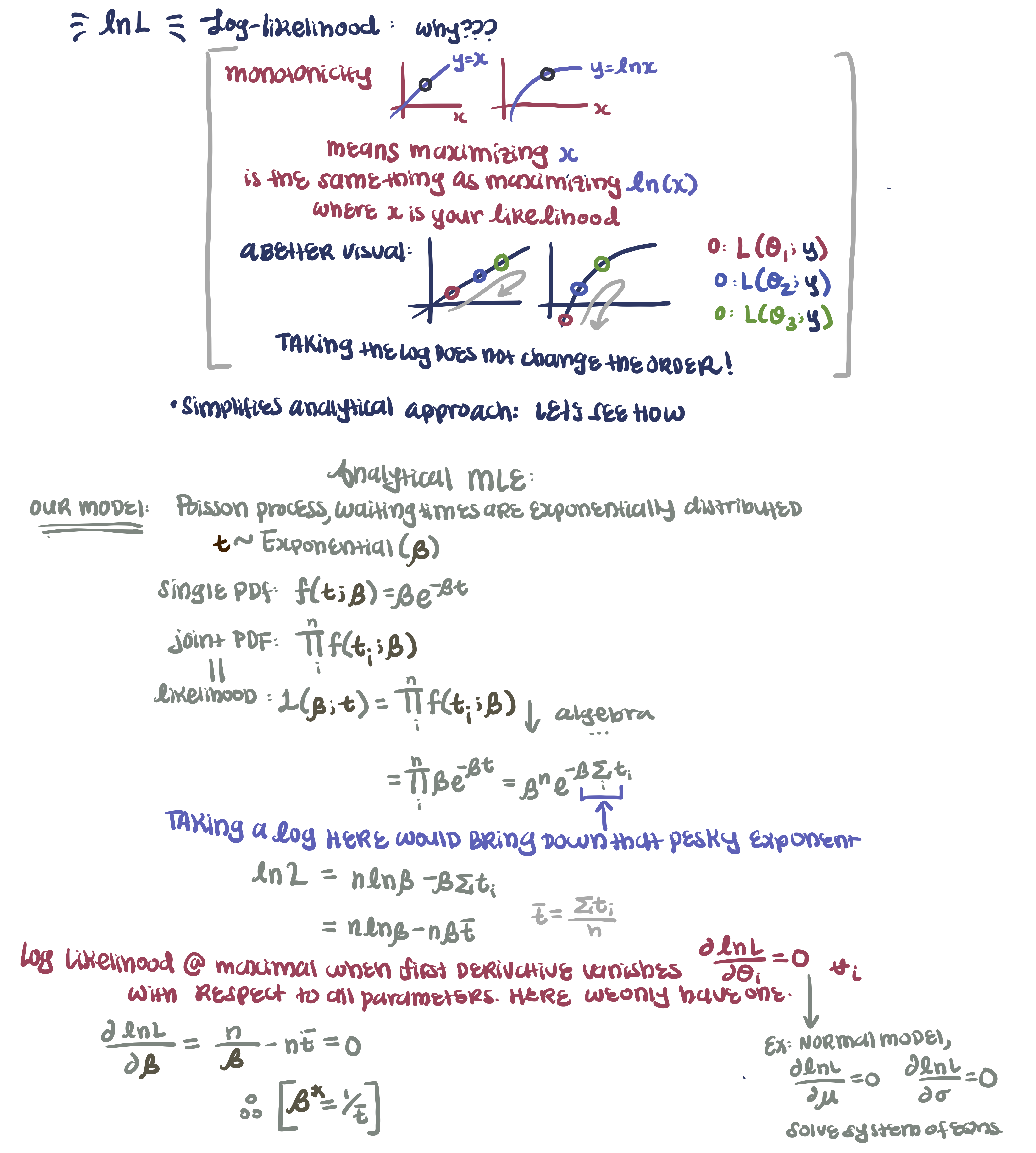
R1. Review of MLE
This recitation was prepared by Rosita Fu.
We’ll review how to actually perform MLE analytically and numerically, and use these methods to construct confidence intervals for our parameters.
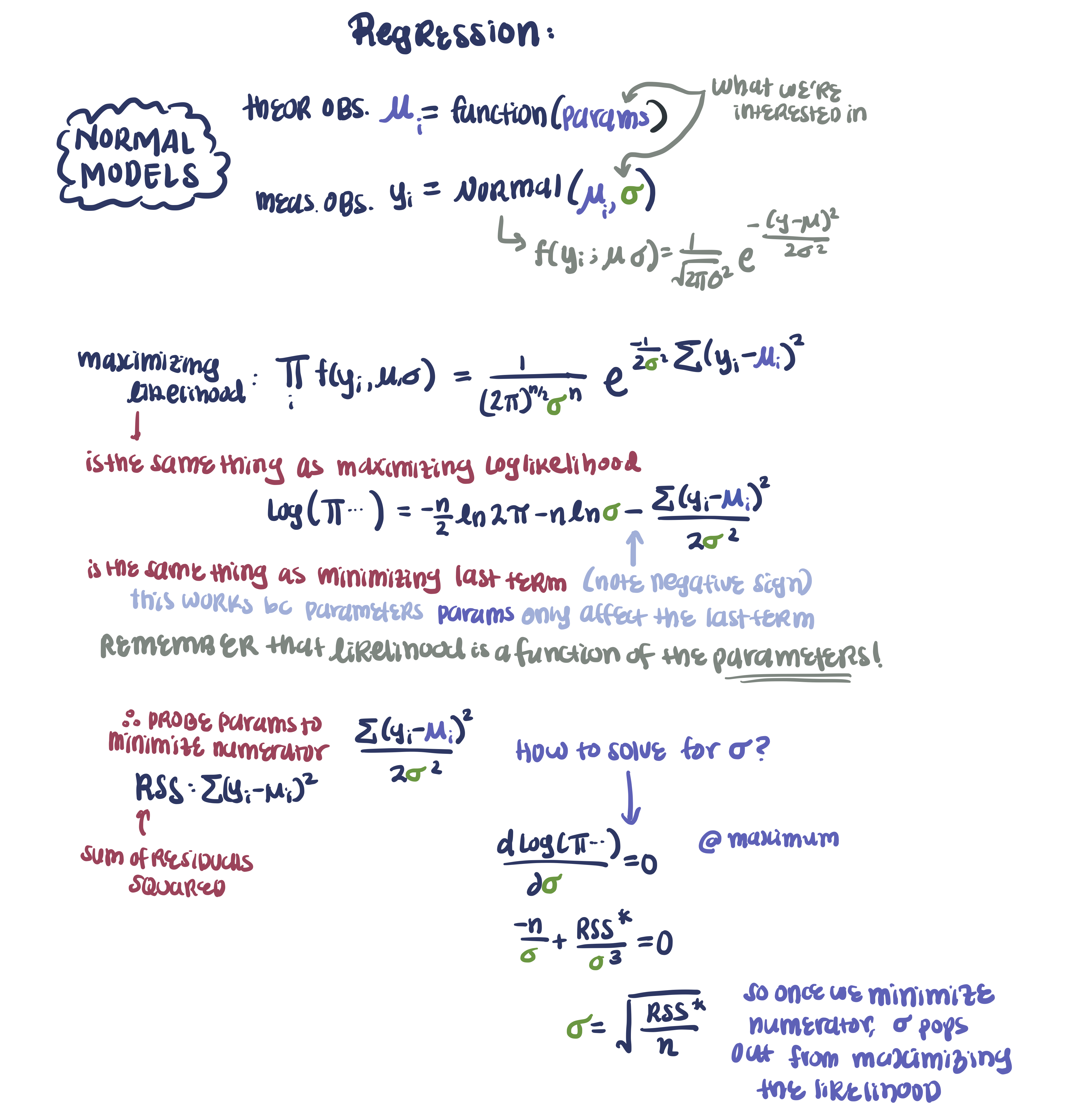
Numerical MLE for mortals tend to be somewhat challenging, so we are always on the look-out for more elegant approaches. For normal distributions, we will apply a very nice property that maximizing its likelihood is functionally equivalent to minimizing the residuals. We will do the math together.
Review of BE/Bi 103 a lessons
The relevant BE/Bi103a lessons are linked, but they are essentially lessons 17, 18, and 20.
MLE Introduction: notes
Numerical MLE: notes
MLE Confidence Intervals: notes
Regression: normal MLE & regression
For those who are just joining us this term, if time allows, to understand confidence intervals, it might be helpful to review what bootstrapping is. If the distributions themselves are new to you, you will become intimately familiar with them by the end of this term, so I wouldn’t worry too much. I would recommend bookmarking distribution-explorer.github.io, or visiting the link so many times all you have to do is type ‘d’ + ‘enter’.
Our mathematical journey will be slightly different this term, but to reach the same state of enlightenment as your peers, it would be nice to compare how confidence intervals and likelihood estimates compare to credible intervals and parameter optimizations later on.
def log_likelihood(...) function that works. 2. Write a scipy.optimize.minimize(...) function with kywargs: fun: lambda parametersx0: initial guess for parameters of type array, (order should match the log_likelihood function you defined)method: either ‘BFGS’ or ‘Powell’ 3. Add warning-filters and retrieve parameters

