R6. Practice model building
This recitation was prepared by Ariana Tribby
The goal of this recitation is to practice coming up with a generative likelihood, identifying which parameters to estimate, and writing down the priors for those parameters.
This recitation will present a series of proposed experiments/scenarios for which you can practice writing full generative models for (priors and likelihoods). The format of each exercise is paper/pencil sketch. Sketching your model before jumping to the code can be really helpful and is great practice! The goal of each exercise is to write your model in the format you’ve seen in lectures, for example, from “MCMC diagnostics” lecture:
\begin{align} &\log_{10} \alpha \sim \text{Norm}(0, 1), \\[1em] &\log_{10} b \sim \text{LogNorm}(2, 1), \\[1em] &\beta = 1/b,\\[1em] &n_i \sim \text{NegBinom}(\alpha, \beta) \;\forall i. \end{align}
Writing your model in this format sets you up for an easier transfer of your knowledge into Stan. Note that you should come up with concrete distributions and values for your priors for these exercises. You are free to use the distribution explorer to help come up with the likelihoods and priors.
Before we start… how do I know which “nomial” to use as a likelihood?
What is the difference between binomial and negative binomial “stories”? How do I know which one to use?
Both are based on independent Bernoulli trials with fixed probability of success, \(\theta\). The number of successes observed in n trials is binomially distributed. The number of trials until the ith success is observed is negative binomially distributed. The number of failures until the ith success (instead of the trials until ith success) is also negative binomially distributed.
[1]:
# Colab setup ------------------
import os, sys, subprocess
if "google.colab" in sys.modules:
    cmd = "pip install --upgrade bebi103 watermark"
    process = subprocess.Popen(cmd.split(), stdout=subprocess.PIPE, stderr=subprocess.PIPE)
    stdout, stderr = process.communicate()
    data_path = "https://s3.amazonaws.com/bebi103.caltech.edu/data/"
else:
    data_path = "../data/"
# ------------------------------

import pandas as pd
import numpy as np
import scipy.stats as st

import bokeh.io
bokeh.io.output_notebook()

import holoviews as hv
import bebi103
hv.extension('bokeh')


Modeling exercises
Try these yourself before looking at solutions at the end of the document!
Exercise 1
You developed a new therapy for cancer that is believed to have 10% probability to cure a patient. The drug does not have any known lethal side effects. You conducted a clinical trial on 500 patients. Fortunately, 75 patients responded positively to the drug. Was this due to chance or other factors such as the therapy or the patient group?
Exercise 2
A certain predator must capture a minimum number of prey before it can grow large enough to reproduce. Other studies have estimated that number to be about 10. What is the mean age of onset of reproduction, given that there is a probability of capturing prey on any given day?
Exercise 3
Ronny, a typical wizard from the Wizarding World is immortal using magic. They are shy and have not been on a date in centuries. Valentine’s Day is fast approaching and Ronny wishes to get out there and go on a date (finally). Before Ronny puts in all of the effort of finding a date, they want to know how successful they might be.
Ronny will look for dates within Wizard Town, which they estimate to have 100 available dates. Ronny’s plan is to go door to door and ask each potential date if they will be their Valentine! <3
First scenario: Ronny believes they are bound to get a “yes” the more potential dates they ask. Build a generative model for the time it might take for Ronny to get a date.
Second scenario: Ronny reveals they are acquaintances with 20 out of the 100 wizards. Having met them before might make them more likely to say yes. Determine what Ronny’s chances are using this new information in a generative model. Ronny asks you what their chances are of a success rate greater than 50%. (Use the distribution explorer).
Exercise 4
This exercise is adapted from Ge 118 with Victor Tsai.
The 3-D equation that relates the arrival time of an earthquake from a measurement station to its epicenter is
\begin{align} t_i = t_s + \frac{\sqrt{(x_s - x_i)^2 + (y_s - y_i)^2 + (z_s - z_i)^2}}{v}. \end{align}
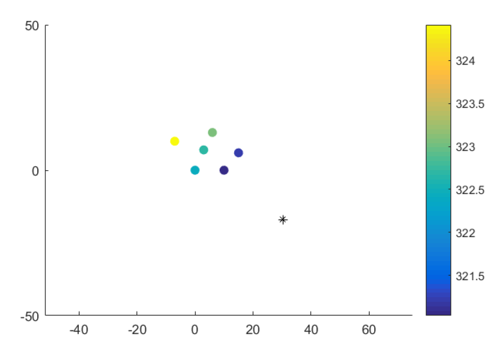
Where i subscripts represent the station measurement location, and s represents the earthquake’s time and location. Below is a plot of measurements taken at stations near the earthquake epicenter.
[2]:
df = pd.DataFrame()
df['xi'] = np.array([0, 10, 15, 6, -7, 3])
df['yi'] = np.array([0, 0, 6, 13, 10, 7])
df['zi'] = np.array([0, 0, 0, 0, 0, 0])
df['ti'] = np.array([322.418, 321.031, 321.228, 323.093, 324.415, 322.706])

hv.Points(
    data=df,
    kdims=['xi','yi'],
    vdims=['ti']
).opts(
    colorbar=True,
    color='ti',
    padding=.1,
    size=10,
    cmap='Viridis',
    ylabel='latitude',
    xlabel='longitude',
    clabel='time'
)
Data type cannot be displayed:
[2]:
This shows how the earthquake “wave” passed through the measurement centers. The goal is to estimate where the epicenter of the earthquake is. Build a generative model.
Solutions (sample solutions, there is no single right answer)
Only look at the solutions after you’ve attempted to sketch the generative model for the exercises yourself!
Exercise 1
We have a fixed probability of success, and a set of N Bernoulli trials (a Bernoulli distribution is parametrized by a single value, \(\theta\), the probability that the trial is successful). We are interested in modeling the number of successes, n, observed in N Bernoulli trials. We can say the data will be binomially distributed. We thus choose a binomial distribution as our likelhood, which means we need to define priors for parameters \(\theta\), the probability of a success, and N, the number of trials. In the problem statement, we were given that the probability of success is estimated to be 10%. To stay on units of percentage, we can use a distribution with small tails that allows values between 0 and less than 100%, with the majority of the probability near zero, so we can use a Beta distribution with a peak near 0.1. The number of trials, \(N\), is given by the data. Thus, our generative model may look like this:
\begin{align} &\theta = \text{Beta}(1.5, 8), \\[1em] & N = 500 \\[1em] &n_i \sim \text{Binom}(N, \theta) \;\forall i. \end{align}
Exercise 2
We have a fixed probability of success, and a set of N Bernoulli trials until the predator is successful. We can model this problem as a number of trials until the success of onset of reproduction. Thus, a negative binomial likelihood would be fitting. This can also be viewed as the number of failures until success of reproduction. We have two parameters: \(\alpha\) and \(\beta\). The desired number of successes is represented by \(\alpha\), and each trial has a probability of \(\beta/(1+\beta)\). Here, \(\alpha\) represents the number of meals needed to grow large enough to reproduce. The the number of failures, y before we get \(\alpha\) success is NB distributed.
We can estimate the number of successes and failures per day, and from there, get the mean age of reproduction (that we won’t do).
We know a priori from other studies the number of meals typically eaten before maturity is about 10. So we will define a broad prior.
The probability of capturing prey on any given day is represented by \(\beta\). The prior distribution should be peaked at low values of \(\beta\). Since we are expressing this as a percentage per day, we are limited from 0 - 100%, so we don’t need large tails. We will use a half normal.
\begin{align} \alpha \sim \text{Halfnorm}(0, 20), \\[1em] \beta \sim \text{Halfnorm}(0, 0.5), \\[1em] Y_i \sim \text{NegBinom}(\alpha, \beta) \;\forall i. \end{align}
Exercise 3
Scenario 1: We are interested in the time it will take to get a date. Ronny suggests that the more people they ask, the more likely they are to say yes. A Weibull distribution describes waiting times for an arrival for a process, and the longer we have waited, the more likely the event is to arrive.
There are two parameters, \(\alpha\), which dictates the shape of the curve, and \(\sigma\), which dictates the rate of arrivals of the event. We don’t know if \(\alpha\) is strictly 1, since perhaps a friend would help Ronny and that might result in more than one step for the date to happen, i.e. more than a single event would result in Ronny having a date. Let’s keep it weakly informative. I used the distribution explorer to find an estimate for sigma, to keep the shape centered at the middle, since I doubt more than 4 outside events other than Ronny asking door to door would be necessary.
\begin{align} \alpha \sim \text{Halfnorm}(0, 3), \\[1em] \sigma \sim \text{Halfnorm}(0, 5), \\[1em] time_i \sim \text{Weibull}(\alpha, \sigma), \\[1em] \end{align}
Scenario 2: The clue here is that we wish to model the probability, and we also know that 20 percent of the possibilities are more likely to result in a date. The beta distribution fits this story. We can think of \(\alpha\) -1 as the number of successes and \(\beta\) -1 as the number of failures. Since we think 20 percent will be successes, then we will center \(\alpha\) around 20, with a small variability, and \(\beta\) around 80.
\begin{align} \alpha \sim \text{Norm}(20, 2), \\[1em] \beta \sim \text{Norm}(80, 2), \\[1em] p_i \sim \text{Beta}(\alpha, \beta), \\[1em] \end{align}
Based on the CDF using the distribution explorer, the probability that the success rate is larger than 50 percent is 20 percent.
Also, this was helpful: https://towardsdatascience.com/beta-distribution-intuition-examples-and-derivation-cf00f4db57af
[3]:
hv.Curve(
    (np.linspace(0, 50, 400), st.norm.pdf(np.linspace(0, 50, 400), 20, 2))
).opts(xlabel = 'alpha')
Data type cannot be displayed:
[3]:
Exercise 4
Just by looking at the equation for t_i, we see that we have 5 parameters to estimate: t_s, x_s, y_s, z_s, and v. For simplicity, we will assume no correlation between stations, but allow for measurement variability between station measurements. We will assume no bias of a certain station - ie homoschedasticity (same error prior each station).
A google search on Wikipedia shows that P-waves have an average velocity of 6km/s, which informs my prior for v.
For time prior: The station data reported about 5 minutes. At the P-wave velocity, that would mean about 1800 km away or about 1,000 miles. The U.S. is almost 3,000 miles across or about 4,500 km. At the 6km/s rate, that would give 750s to travel across the U.S. I think this would be plenty upper limit, since people in D.C. can’t feel earthquakes coming from L.A.
For x_s and y_s: delta longitude covered by the US is 50 degrees. Based on our reasoning for time, it should not be farther than this. We notice from the station data that the earthquake is coming from the bottom right. I will just pick 0 degrees longitude (near the median of the stations) and then get 45 degrees longitude on the right side. Same reasoning for latitude, except we can’t say for sure whether the earthquake is above or below the median of the stations. I will choose a normal instead.
For z_s: typical earthquakes range from 0 - 700 km in depth according to a Google search.
For sigma, I highly doubt there would be more of a couple minutes in measurement variability between stations. It would be troubling if that were the case.
\begin{align} &t_i = t_s + \frac{\sqrt{(x_s - x_i)^2 + (y_s - y_i)^2 + (z_s - z_i)^2}}{v}\\ &v \sim \text{HalfNorm}(10)\\ &t_s \sim \text{HalfNorm}(700)\\ &x_s \sim \text{HalfNorm}(45)\\ &y_s \sim \text{Norm}(5,45)\\ &z_s \sim \text{HalfNorm}(700)\\ &\sigma \sim \text{HalfNorm}(60)\\ &t_{station} \sim \text{Norm}(t_i, \sigma)\\ \end{align}
I haven’t run this model, but I did a least squares a couple of years ago (that assumes uniform prior distributions) and no station variability and I got this result:
[ ]: